I could not get autoplot to work with the GDP data frame. I have never used autoplot but it seems you must define a method for that kind of object. I did plot the time series Y and found that the x values are large negative numbers because the data are plotted as being in the year 1.
GDP <- structure(list(DATE = c("1/1/1947", "4/1/1947", "7/1/1947", "10/1/1947",
"1/1/1948", "4/1/1948"),
GDP = c(2033.061, 2027.639, 2023.452, 2055.103, 2086.017, 2120.45)),
class = c("tbl_df", "tbl", "data.frame"), row.names = c(NA, -6L))
library(ggplot2)
library(ggfortify)
Y <- ts(GDP$GDP, start(1947,1), frequency = 4)
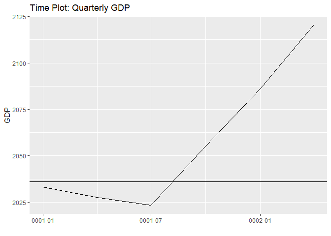
PLT <- autoplot(Y) +
ggtitle("Time Plot: Quarterly GDP") +
ylab("GDP")
#The dates are in year 1
PLT$data$Index
#> [1] "0001-01-01" "0001-04-01" "0001-07-01" "0001-10-01" "0002-01-01"
#> [6] "0002-04-01"
#Their numeric value is ~ -719162, the number of days between Jan 1, 1970 and Jan 1, 1
as.numeric(PLT$data$Index)
#> [1] -719162 -719072 -718981 -718889 -718797 -718707
autoplot(Y) +
ggtitle("Time Plot: Quarterly GDP") +
ylab("GDP") + geom_abline(slope = 1/-719162, intercept = 2035)
That may not be very helpful because you seem to be able to plot the GDP data frame. Try storing the result of autoplot in a variable PLT as I did above and look at the value of
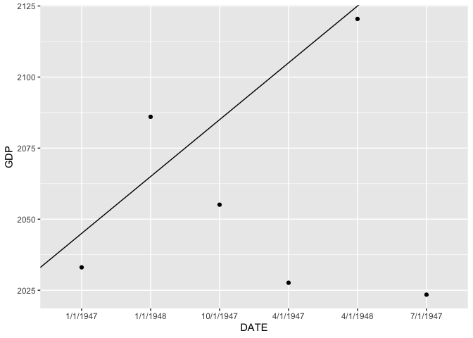
Yeah, I was getting the same results. The only way I came up to figure it out was to not use the data as a time series object and replace the date with an order like this:
GDP["order"] <- seq(1,290)
# run regression
lr <- lm(log(GDP)~order, data = GDP)
# scatter plot
p <- ggplot(GDP, aes(x=order, y=log(GDP)))+geom_point()
# fitted line plot
p + geom_abline(intercept = lr$coefficients[1], slope = lr$coefficients[2])