Plotting a Mean Heart Rate Over Specific Time Points

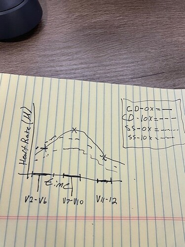
I'm expanding on a previous conversation (Reference to other post). I'm having trouble figuring out how to grab a mean for a group of specific ID numbers across different units of time within my data. For example, if I wanted to take CD-01 through CD-09 & CD-11 across V2 to V6 and plot that mean, then take V7 through V10 and plot that then V11 and V12 and the same thing. Then do that again for CD-103 and 105 and the SS etc. I suppose I still have to keep the data frame in long but I'm struggling with the data management part like selecting the columns.

So basically a mean plot that across at different points in the data set. Any information would be helpful. Thank you

heartrate <- tibble::tribble(
                       ~V1,  ~V2,  ~V3,  ~V4,  ~V5,  ~V6,  ~V7,  ~V8,  ~V9, ~V10, ~V11, ~V12,
               "ID Number",   0L,   1L,   2L,   3L,   4L,   5L,   6L,   7L,   8L,   9L,  10L,
                   "CD-01",  66L,  66L,  64L,  64L,  58L,  58L,  58L,  57L,  56L,  56L,  57L,
                   "SS-02",  85L,  84L,  83L,  81L,  80L,  79L,  78L,  78L,  79L,  80L,  80L,
                   "CD-03", 103L, 103L, 103L, 103L, 103L, 103L, 103L, 103L, 103L, 103L, 103L,
                   "CD-04", 115L, 115L, 114L, 114L, 114L, 114L, 112L, 111L, 110L, 109L, 109L,
                  "SS-101",  63L,  63L,  63L,  63L,  77L,  78L,  80L,  77L,  76L,  67L,  67L,
                   "CD-05",  84L,  63L,  62L,  62L,  63L,  58L,  58L,  54L,  62L,  66L,  66L,
                  "SS-102",  49L,  48L,  46L,  46L,  45L,  46L,  45L,  45L,  45L,  45L,  46L,
                  "CD-103",  70L,  69L,  68L,  68L,  69L,  69L,  69L,  69L,  68L,  69L,  70L,
                   "CD-06",  83L,  84L,  84L,  84L,  84L,  84L,  82L,  82L,  82L,  82L,  81L,
                   "SS-08",  79L,  78L,  67L,  67L,  68L,  62L,  62L,  62L,  63L,  72L,  72L,
                   "CD-09", 240L, 202L, 141L, 106L,  89L,  74L,  71L,  71L,  71L,  72L,  74L,
                   "SS-10",  78L,  78L,  77L,  76L,  75L,  75L,  75L,  75L,  76L,  76L,  76L,
                  "CD-105",  66L,  66L,  66L,  66L,  66L,  66L,  67L,  67L,  67L,  67L,  68L,
                   "CD-11",  66L,  66L,  76L,  76L,  76L,  77L,  75L,  75L,  75L,  75L,  76L
               )
head(heartrate)
Hi @nviet
I'll answer at least the first part of your question.
There are a few concepts of tidy data to address:

  • observations (time element) must be in rows, not columns
  • variables (your categories) must be in columns, not in rows
    --> so we need to transpose
  • since categories ((CD-01, SS-02, ...) will become variables, they need to be valid R variable names to avoid using backticks
#create a named vector to clean up variable names, in a standard tidyverse format
# this will be used in the second code chunk
var_names <- heartrate %>% transmute(clean_names = str_replace(V1, "[ -]", "_"), old_names = c(1:nrow(.))) %>% 
  deframe()
# transform your initial tibble into a tidy format
heartrate2 <- heartrate %>% 
  # transpose (1 observation per row, one column per category) and 
  t() %>%
  # transposing turns your tibble into a matrix, it needs to be re-tibbled
  as_tibble() %>% 
  # changing variable names from the name vector
  # more info here if you'd like: https://forum.posit.co/t/rename-with-a-named-vector-list-and-contribution-to-the-tidyverse/2383
  rename(!!! var_names) %>% 
  # remove first row that was "pushed" to variable names
  slice(-1) %>% 
  # transposing your initial tibble that contained all integers except the V1 variable coerced the matrix to be characters
  # now that we have no character variable in the tibble, we convert all to integer again
  mutate_all(as.integer) %>% 
  # I add a new "time" column that will help when plotting (personal choice)
  mutate(time = str_c("t", 1:nrow(.))) %>% 
  # convert to long format that is ggplot-friendly
  pivot_longer(CD_01:CD_11, names_to = "category", values_to = "value") 

# now you can plot the usual way
heartrate2 %>% 
  ggplot(aes(x = fct_reorder(time, ID_Number), y = value, group = category, color = category)) + 
  geom_line() + 
  labs(x = "time", y = "heart rate")

# or alternatively
heartrate2 %>% 
  ggplot(aes(x = fct_reorder(time, ID_Number), y = value, group = category, color = category)) + 
  geom_line() + 
  labs(x = "time", y = "heart rate") + 
  facet_wrap(~category)

I hope this helps with part of your question.

Thank you for your help but this doesn't do much to address the question. If you look at the reference to the other post this was kind of addressed already. I sincerely appreciate it though.

Last attempt before the weekend, I hope this is closer to what you're loking for, grouped the categories into 4 main groups, calculate mean of each per time time element and plotted:

heartrate3 <- heartrate %>% 
  t() %>%
  as_tibble() %>% 
  rename(!!! var_names) %>% 
  slice(-1) %>% 
  mutate_all(as.integer) %>% 
  mutate(time = str_c("t", 1:nrow(.)), .before = ID_Number) %>%
  pivot_longer(CD_01:CD_11, names_to = "category", values_to = "value") %>% 
  mutate(main_group = case_when(
    str_detect(category, "CD_0") ~ "CD_0x",
    str_detect(category, "CD_1") ~ "CD_1x",
    str_detect(category, "SS_0") ~ "SS_0x",
    str_detect(category, "SS_1") ~ "SS_1x"
  )) %>% 
  group_by(main_group, time) %>% 
  summarize(mean_group = mean(value)) %>% 
  mutate(ID_Number = as.numeric(str_remove(time, "t")))

heartrate3 %>% 
  ggplot(aes(x = fct_reorder(time, ID_Number), y = mean_group, group = main_group, color = main_group)) + 
  geom_line() + 
  labs(x = "time", y = "heart rate")

I hope this is getting closer.

This might be it.

The "str_detect(category, "CD_0")~"CD_0x", I assuming (in layman terms) selected all the cases with CD_0 to CD_0X(X being the maximum number in the data set as long as there is a "CD_0" in front of the following number)?

Yes, that's the spirit, for example str_detect("CD_0656468154dofjhosf", "CD_0") will return TRUE, thus validating the first condition in the case_when statements.
I added something in the case_when function, when a category doesn't match any of the 4 patterns we defined, then it will have a fallback value of "other category" that will appear in your plot.
I copied the whole block below with the add-on.

Also note that what is in the str_detect() arguments is a very basic regex that works on the data that you shared, if you have much more data with different patterns, it could be worth making the expressions a bit more solid. But this part you will be able to diagnose if you ever see the "other category" line in your plot.

heartrate3 <- heartrate %>% 
  t() %>%
  as_tibble() %>% 
  rename(!!! var_names) %>% 
  slice(-1) %>% 
  mutate_all(as.integer) %>% 
  mutate(time = str_c("t", 1:nrow(.)), .before = ID_Number) %>%
  pivot_longer(CD_01:CD_11, names_to = "category", values_to = "value") %>% 
  mutate(main_group = case_when(
    str_detect(category, "CD_0") ~ "CD_0x",
    str_detect(category, "CD_1") ~ "CD_1x",
    str_detect(category, "SS_0") ~ "SS_0x",
    str_detect(category, "SS_1") ~ "SS_1x", 
    TRUE ~ "other category"
  )) %>% 
  group_by(main_group, time) %>% 
  summarize(mean_group = mean(value)) %>% 
  mutate(ID_Number = as.numeric(str_remove(time, "t")))

This topic was automatically closed 21 days after the last reply. New replies are no longer allowed.

If you have a query related to it or one of the replies, start a new topic and refer back with a link.