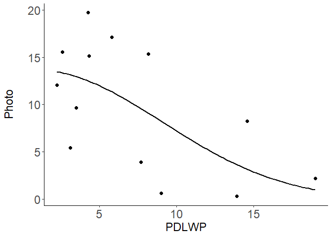
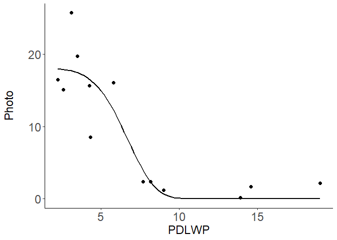
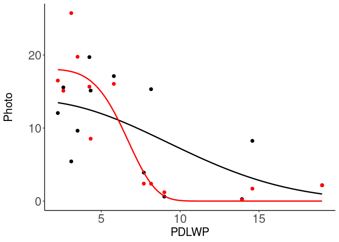
Plotting 2 weibull curves in a single plot using nls2 and ggplot2

Hello,
I would like to plot two 3-parameter Weibull curves in a single plot. I know how to plot individual curves using nls2 and ggplot2. My problem is, that I don’t know how to plot two curves from two data groups in the same plot. In the example below I would like to define the Weibull parameters for the data points belonging to the group “dip1” (in column “geno”) and for the group “dip2” with the “nls(…) command. I then would like to plot two individual curves using ggplot2 in the same plot. In this small example, my X-axis points are called “PDLWP” and my Y-axis points are called “Photo”. I already wrote some code that plots a single Weibull curve using the combined data sets of dip1 and dip2 points. Could anybody help me to plot two curves one for dip1 and one for dip2? Thank you very much for your help

dta<-structure(list(ploidy = c("dip", "dip", "dip", "dip", "dip", "dip", "dip", "dip", "dip", "dip", "dip", "dip", "dip", "dip", "dip", "dip", "dip", "dip", "dip", "dip", "dip", "dip", "dip", "dip", "dip", "dip"), geno = c("dip1", "dip1", "dip1", "dip1", "dip1", "dip1", "dip1", "dip1", "dip1", "dip1", "dip1", "dip1", "dip1", "dip2", "dip2", "dip2", "dip2", "dip2", "dip2", "dip2", "dip2", "dip2", "dip2", "dip2", "dip2", "dip2"), Photo = c(5.429849559, 15.56020359, 17.11031242, 3.898958096, 2.170068415, 9.635005028, 19.71198385, 0.621534066, 15.31952903, 12.05323573, 0.268807378, 15.12996082, 8.24572244, 25.73923074, 15.10455617, 16.04850297, 2.390612635, 2.164994013, 19.75451088, 15.65863235, 1.206895049, 2.374035234, 16.50051398, 0.16242929, 8.537029628, 1.700498836 ), PDLWP = c(3.1, 2.6, 5.8, 7.7, 19, 3.5, 4.25, 9, 8.16, 2.25, 13.92, 4.33, 14.58, 3.1, 2.6, 5.8, 7.7, 19, 3.5, 4.25, 9, 8.16, 2.25, 13.92, 4.33, 14.58)), class = "data.frame", row.names = c(NA, -26L))
dta
#>    ploidy geno      Photo PDLWP
#> 1     dip dip1  5.4298496  3.10
#> 2     dip dip1 15.5602036  2.60
#> 3     dip dip1 17.1103124  5.80
#> 4     dip dip1  3.8989581  7.70
#> 5     dip dip1  2.1700684 19.00
#> 6     dip dip1  9.6350050  3.50
#> 7     dip dip1 19.7119838  4.25
#> 8     dip dip1  0.6215341  9.00
#> 9     dip dip1 15.3195290  8.16
#> 10    dip dip1 12.0532357  2.25
#> 11    dip dip1  0.2688074 13.92
#> 12    dip dip1 15.1299608  4.33
#> 13    dip dip1  8.2457224 14.58
#> 14    dip dip2 25.7392307  3.10
#> 15    dip dip2 15.1045562  2.60
#> 16    dip dip2 16.0485030  5.80
#> 17    dip dip2  2.3906126  7.70
#> 18    dip dip2  2.1649940 19.00
#> 19    dip dip2 19.7545109  3.50
#> 20    dip dip2 15.6586323  4.25
#> 21    dip dip2  1.2068950  9.00
#> 22    dip dip2  2.3740352  8.16
#> 23    dip dip2 16.5005140  2.25
#> 24    dip dip2  0.1624293 13.92
#> 25    dip dip2  8.5370296  4.33
#> 26    dip dip2  1.7004988 14.58
#Load packages
library(ggplot2)
library(nlme)
library(nls2)
library(proto)

#model structure: 3 parameter Weibull
#y ~ m*exp(-1*(x/b)^c)

#Define the outer boundaries to search for initial values
grd <- data.frame(m=c(10,30),
                  b=c(0,10),
                  c=c(0,10))

#Brute-force initial values
fit <- nls2(Photo ~ m*exp(-1*(PDLWP/b)^c),
            data=dta,
            start = grd,
            algorithm = "brute-force",
            control=list(maxiter=10000))
fit
#> Nonlinear regression model
#>   model: Photo ~ m * exp(-1 * (PDLWP/b)^c)
#>    data: dta
#>      m      b      c 
#> 14.762  8.095  7.619 
#>  residual sum-of-squares: 583.4
#> 
#> Number of iterations to convergence: 10648 
#> Achieved convergence tolerance: NA
finalfit <- nls(Photo ~ m*exp(-1*(PDLWP/b)^c), data=dta, start=as.list(coef(fit)))

# Plot in ggplot
example<-ggplot(dta, aes(x=PDLWP,y=Photo)) + geom_point(size=2)+
  theme_classic()+
  theme(legend.position="none")+
  theme(axis.text=element_text(size=18),
        axis.title=element_text(size=17,),axis.title.y=element_text(margin=margin(0,20,0,0)))+
  stat_smooth(method = "nls", formula = y ~ m*exp(-1*(x/b)^c), method.args=list(start=as.list(coef(finalfit))), size = 0.9, se = FALSE, colour = "black")

example
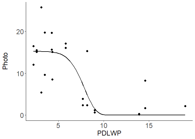
Created on 2021-03-03 by the reprex package (v1.0.0)
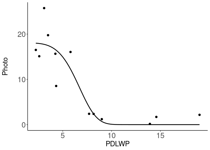
Your example doesn't run. Please provide a reproducible example that runs. That includes loading the packages.

1 Like

See the FAQ: How to do a minimal reproducible example reprex for beginners.

Hi. Thank you for your responses. I cleaned the code and added the necessary packages.
It should work now.
BTW: "reprex" is pretty neat. I was not aware of that before

That helps and runs the code. However, I'm unsure of your intent. The geno variable plays no role in example, which depends solely on model: Photo ~ m * exp(-1 * (PDLWP/b)^c) in geom_stat.

Every R problem can be thought of with advantage as the interaction of three objects— an existing object, x , a desired object,y , and a function, f, that will return a value of y given x as an argument. In other words, school algebra— f(x) = y. Any of the objects can be composites.

Here we seem to have all the pieces but for the function that transforms dta. Are you looking to combine the results of the script on separate subsets, one restricted to only dip1 and the other to dip2? That would mean a ggplot(dta, aes(x = PDLWP, y = Photo)) object as base with two finalfit objects (one for each subset). Is that the intended result?

Hi Technocrat,
I would like to fit a weibull curve to only the subest of dip1 and another weibull curve to the subest of dip2 data.
This would mean that I would get 2 different sets of curve estimates for "m", "b" and "c" (in my example I caluclated "m", "b" and "c" for the combined dip1 and dip2 data sets and fit a curve to the enitre data set. However, this is not what I am interested in. It should just be the basis for the next step).
Finally I would like to plot the dip1 and dip2 curve in the same plot using ggplot2.

A post was split to a new topic: web-scraping and rvest help

dip2 works, but dip1 produces a singular gradient; will need separate grd for each.

suppressPackageStartupMessages({
  library(dplyr)
  library(ggplot2)
  library(nls2)
})

dta <- data.frame(
  geno = c("dip1", "dip1", "dip1", "dip1", "dip1", "dip1", "dip1", "dip1", "dip1", "dip1", "dip1", "dip1", "dip1", "dip2", "dip2", "dip2", "dip2", "dip2", "dip2", "dip2", "dip2", "dip2", "dip2", "dip2", "dip2", "dip2"),
  Photo = c(5.429849559, 15.56020359, 17.11031242, 3.898958096, 2.170068415, 9.635005028, 19.71198385, 0.621534066, 15.31952903, 12.05323573, 0.268807378, 15.12996082, 8.24572244, 25.73923074, 15.10455617, 16.04850297, 2.390612635, 2.164994013, 19.75451088, 15.65863235, 1.206895049, 2.374035234, 16.50051398, 0.16242929, 8.537029628, 1.700498836),
  PDLWP = c(3.1, 2.6, 5.8, 7.7, 19, 3.5, 4.25, 9, 8.16, 2.25, 13.92, 4.33, 14.58, 3.1, 2.6, 5.8, 7.7, 19, 3.5, 4.25, 9, 8.16, 2.25, 13.92, 4.33, 14.58))

dta %>% filter(geno == "dip1") -> dip1
dta %>% filter(geno == "dip2") -> dip2

grd <- data.frame(
  m = c(10, 30),
  b = c(0, 10),
  c = c(0, 10)
)

fit_2 <- nls2(Photo ~ m * exp(-1 * (PDLWP / b)^c),
  data = dip2,
  start = grd,
  algorithm = "brute-force",
  control = list(maxiter = 10000)
)

finalfit_2 <- nls(Photo ~ m * exp(-1 * (PDLWP / b)^c), data = dip2, start = as.list(coef(fit_2)))

example <- ggplot(dip2, aes(x = PDLWP, y = Photo)) +
  geom_point(size = 2) +
  theme_classic() +
  theme(legend.position = "none") +
  theme(
    axis.text = element_text(size = 18),
    axis.title = element_text(size = 17, ), axis.title.y = element_text(margin = margin(0, 20, 0, 0))
  ) +
  stat_smooth(method = "nls", formula = y ~ m * exp(-1 * (x / b)^c), method.args = list(start = as.list(coef(finalfit_2))), size = 0.9, se = FALSE, colour = "black")

example

Hi Technocrat,
I could figure out a way to calculate and individually plot my curves (see code)

dta<-structure(list(ploidy = c("dip", "dip", "dip", "dip", "dip", "dip", "dip", "dip", "dip", "dip", "dip", "dip", "dip", "dip", "dip", "dip", "dip", "dip", "dip", "dip", "dip", "dip", "dip", "dip", "dip", "dip"), geno = c("dip1", "dip1", "dip1", "dip1", "dip1", "dip1", "dip1", "dip1", "dip1", "dip1", "dip1", "dip1", "dip1", "dip2", "dip2", "dip2", "dip2", "dip2", "dip2", "dip2", "dip2", "dip2", "dip2", "dip2", "dip2", "dip2"), Photo = c(5.429849559, 15.56020359, 17.11031242, 3.898958096, 2.170068415, 9.635005028, 19.71198385, 0.621534066, 15.31952903, 12.05323573, 0.268807378, 15.12996082, 8.24572244, 25.73923074, 15.10455617, 16.04850297, 2.390612635, 2.164994013, 19.75451088, 15.65863235, 1.206895049, 2.374035234, 16.50051398, 0.16242929, 8.537029628, 1.700498836 ), PDLWP = c(3.1, 2.6, 5.8, 7.7, 19, 3.5, 4.25, 9, 8.16, 2.25, 13.92, 4.33, 14.58, 3.1, 2.6, 5.8, 7.7, 19, 3.5, 4.25, 9, 8.16, 2.25, 13.92, 4.33, 14.58)), class = "data.frame", row.names = c(NA, -26L))
dta
#>    ploidy geno      Photo PDLWP
#> 1     dip dip1  5.4298496  3.10
#> 2     dip dip1 15.5602036  2.60
#> 3     dip dip1 17.1103124  5.80
#> 4     dip dip1  3.8989581  7.70
#> 5     dip dip1  2.1700684 19.00
#> 6     dip dip1  9.6350050  3.50
#> 7     dip dip1 19.7119838  4.25
#> 8     dip dip1  0.6215341  9.00
#> 9     dip dip1 15.3195290  8.16
#> 10    dip dip1 12.0532357  2.25
#> 11    dip dip1  0.2688074 13.92
#> 12    dip dip1 15.1299608  4.33
#> 13    dip dip1  8.2457224 14.58
#> 14    dip dip2 25.7392307  3.10
#> 15    dip dip2 15.1045562  2.60
#> 16    dip dip2 16.0485030  5.80
#> 17    dip dip2  2.3906126  7.70
#> 18    dip dip2  2.1649940 19.00
#> 19    dip dip2 19.7545109  3.50
#> 20    dip dip2 15.6586323  4.25
#> 21    dip dip2  1.2068950  9.00
#> 22    dip dip2  2.3740352  8.16
#> 23    dip dip2 16.5005140  2.25
#> 24    dip dip2  0.1624293 13.92
#> 25    dip dip2  8.5370296  4.33
#> 26    dip dip2  1.7004988 14.58
#Load packages
library(ggplot2)
library(nlme)
library(nls2)
#> Lade nötiges Paket: proto
library(proto)

#model structure: 3 parameter Weibull
#y ~ m*exp(-1*(x/b)^c)


#Subset Dip1
dip1dta<-subset(dta,geno=="dip1")
#Define the outer boundaries to search for initial values
grddip1 <- data.frame(m=c(10,30),
                      b=c(0.1,7),
                      c=c(0.1,10))
#Brute-force initial values
fitdip1 <- nls2(Photo ~ m*exp(-1*(PDLWP/b)^c),
                data=dip1dta,
                start = grddip1,
                algorithm = "brute-force",
                control=list(maxiter=10000))
fitdip1
#> Nonlinear regression model
#>   model: Photo ~ m * exp(-1 * (PDLWP/b)^c)
#>    data: dip1dta
#>       m       b       c 
#> 25.2381  6.6714  0.5714 
#>  residual sum-of-squares: 369.2
#> 
#> Number of iterations to convergence: 10648 
#> Achieved convergence tolerance: NA
finalfitdip1 <- nls(Photo ~ m*exp(-1*(PDLWP/b)^c), data=dip1dta, start=as.list(coef(fitdip1)))

# Plot in ggplot
exampledip1<-ggplot(dip1dta, aes(x=PDLWP,y=Photo)) + geom_point(size=2)+
  theme_classic()+
  theme(legend.position="none")+
  theme(axis.text=element_text(size=18),
        axis.title=element_text(size=17,),axis.title.y=element_text(margin=margin(0,20,0,0)))+
  stat_smooth(method = "nls", formula = y ~ m*exp(-1*(x/b)^c), method.args=list(start=as.list(coef(finalfitdip1))), size = 0.9, se = FALSE, colour = "black")

exampledip1


#Subset Dip2
dip2dta<-subset(dta,geno=="dip2")
#Define the outer boundaries to search for initial values
grddip2 <- data.frame(m=c(10,30),
                      b=c(0,10),
                      c=c(0,10))
#Brute-force initial values
fitdip2 <- nls2(Photo ~ m*exp(-1*(PDLWP/b)^c),
                data=dip2dta,
                start = grddip2,
                algorithm = "brute-force",
                control=list(maxiter=10000))
fitdip2
#> Nonlinear regression model
#>   model: Photo ~ m * exp(-1 * (PDLWP/b)^c)
#>    data: dip2dta
#>      m      b      c 
#> 17.619  7.143  5.238 
#>  residual sum-of-squares: 167.9
#> 
#> Number of iterations to convergence: 10648 
#> Achieved convergence tolerance: NA
finalfitdip2 <- nls(Photo ~ m*exp(-1*(PDLWP/b)^c), data=dip2dta, start=as.list(coef(fitdip2)))


# Plot in ggplot
exampledip2<-ggplot(dip2dta, aes(x=PDLWP,y=Photo)) + geom_point(size=2)+
  theme_classic()+
  theme(legend.position="none")+
  theme(axis.text=element_text(size=18),
        axis.title=element_text(size=17,),axis.title.y=element_text(margin=margin(0,20,0,0)))+
  stat_smooth(method = "nls", formula = y ~ m*exp(-1*(x/b)^c), method.args=list(start=as.list(coef(finalfitdip2))), size = 0.9, se = FALSE, colour = "black")

exampledip2

Created on 2021-03-04 by the reprex package (v1.0.0)

The question now is: How can I plot both curves in a single plot ?

suppressPackageStartupMessages({
  library(dplyr)
  library(ggplot2)
  library(nls2)
})

dta <- data.frame(
  ploidy = c("dip", "dip", "dip", "dip", "dip", "dip", "dip", "dip", "dip", "dip", "dip", "dip", "dip", "dip", "dip", "dip", "dip", "dip", "dip", "dip", "dip", "dip", "dip", "dip", "dip", "dip"), geno = c("dip1", "dip1", "dip1", "dip1", "dip1", "dip1", "dip1", "dip1", "dip1", "dip1", "dip1", "dip1", "dip1", "dip2", "dip2", "dip2", "dip2", "dip2", "dip2", "dip2", "dip2", "dip2", "dip2", "dip2", "dip2", "dip2"),
  Photo = c(5.429849559, 15.56020359, 17.11031242, 3.898958096, 2.170068415, 9.635005028, 19.71198385, 0.621534066, 15.31952903, 12.05323573, 0.268807378, 15.12996082, 8.24572244, 25.73923074, 15.10455617, 16.04850297, 2.390612635, 2.164994013, 19.75451088, 15.65863235, 1.206895049, 2.374035234, 16.50051398, 0.16242929, 8.537029628, 1.700498836),
  PDLWP = c(3.1, 2.6, 5.8, 7.7, 19, 3.5, 4.25, 9, 8.16, 2.25, 13.92, 4.33, 14.58, 3.1, 2.6, 5.8, 7.7, 19, 3.5, 4.25, 9, 8.16, 2.25, 13.92, 4.33, 14.58)
)

dip1dta <- subset(dta, geno == "dip1")
# Define the outer boundaries to search for initial values
grddip1 <- data.frame(
  m = c(10, 30),
  b = c(0.1, 7),
  c = c(0.1, 10)
)
# Brute-force initial values
fitdip1 <- nls2(Photo ~ m * exp(-1 * (PDLWP / b)^c),
  data = dip1dta,
  start = grddip1,
  algorithm = "brute-force",
  control = list(maxiter = 10000)
)

finalfitdip1 <- nls(Photo ~ m * exp(-1 * (PDLWP / b)^c), data = dip1dta, start = as.list(coef(fitdip1)))

dip2dta <- subset(dta, geno == "dip2")
# Define the outer boundaries to search for initial values
grddip2 <- data.frame(
  m = c(10, 30),
  b = c(0, 10),
  c = c(0, 10)
)
# Brute-force initial values
fitdip2 <- nls2(Photo ~ m * exp(-1 * (PDLWP / b)^c),
  data = dip2dta,
  start = grddip2,
  algorithm = "brute-force",
  control = list(maxiter = 10000)
)

finalfitdip2 <- nls(Photo ~ m * exp(-1 * (PDLWP / b)^c), data = dip2dta, start = as.list(coef(fitdip2)))

exampledip1 <- ggplot(dta, aes(x = PDLWP, y = Photo, color = geno)) +
  scale_colour_discrete(type = c("black", "red")) +
  geom_point(size = 2) +
  theme_classic() +
  theme(legend.position = "none") +
  theme(
    axis.text = element_text(size = 18),
    axis.title = element_text(size = 17, ), axis.title.y = element_text(margin = margin(0, 20, 0, 0))
  ) +
  stat_smooth(data = dip1dta, mapping = aes(x = PDLWP, y = Photo), method = "nls", formula = y ~ m * exp(-1 * (x / b)^c), method.args = list(start = as.list(coef(finalfitdip1))), size = 0.9, se = FALSE, colour = "black") +
  stat_smooth(data = dip2dta, mapping = aes(x = PDLWP, y = Photo), method = "nls", formula = y ~ m * exp(-1 * (x / b)^c), method.args = list(start = as.list(coef(finalfitdip2))), size = 0.9, se = FALSE, colour = "red")

exampledip1

1 Like

Dear technocrat.
Thank you very much! This is awesome and very much appreciated.

One tiny bit of the code above seems to cause an error.
Instead of

  scale_colour_discrete(type = c("black", "red")) +

I had to write

  scale_colour_manual(values = c("black", "red")) +

Thanks again!

1 Like

When you update ggplot2 to version 3, both will work.

This topic was automatically closed 7 days after the last reply. New replies are no longer allowed.

If you have a query related to it or one of the replies, start a new topic and refer back with a link.