Plot in a box with long text legend in a box

Hi there - I am trying to make a typical figure for a grant, in which we usually have a nice plot with a bounding box, and an adjacent chatty figure legend (usually below) with its own matching bounding box.

An example is shown here
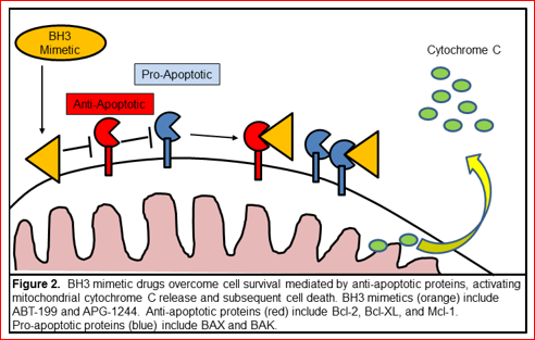
image

Another example with a ggplot is shown here
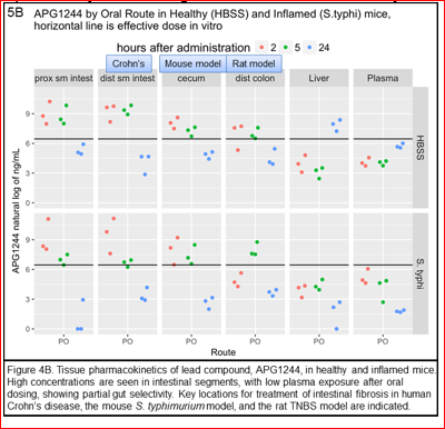
image
Note the mismatch between the tag (upper left) and the figure_legend (5B vs 4B) .

Ideally, I would like to do this programmatically and prevent these kinds of errors.

I have tried a few options, with only modest success.
The plot with a bounding box is pretty straightforward, with
theme(plot.background = element_rect(color='black'))

I would like an easy way to create a auto-wrapping textGrob within a bounding box, with better control of the spacing between lines (lineheight?). There are probably better approaches.

I would also like a better way to put these together, so that the bottom of the plot bounding box overlays the top of the figure_legend bounding box.

Here are things that I have tried in a reprex.

# Goal: plot in box with figure_legend in box below
library(tidyverse)
library(gridExtra)
#> 
#> Attaching package: 'gridExtra'
#> The following object is masked from 'package:dplyr':
#> 
#>     combine
library(grid)
p <- iris %>% 
  ggplot() +
  aes(x= Sepal.Width, y = Sepal.Length) +
  geom_point()

p2 <- p +
  theme(plot.background = element_rect(color='black'))

legend <- "Figure 1. An Amazing Plot. This is a totally awesome plot. It has great properties. The  \n
            points are black. The background is gray. You should definitely fund this grant."


# one option - caption
p2 +
  labs(caption = legend) +
  theme(plot.caption = element_text(size = 12, hjust = 0,
        margin = margin(15,0,0,0)))
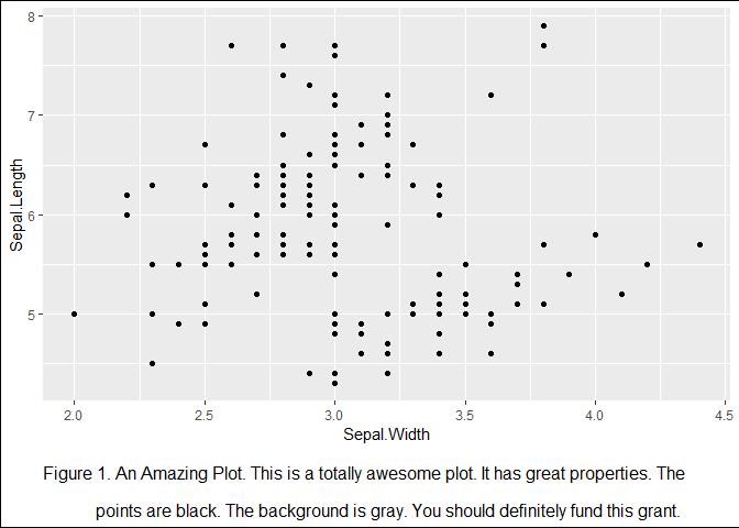

# notes - pretty good, but no dividing line between the plot and the legend
# also need lower lineheight/space between lines


# another option - textGrob
figlegend <- textGrob(legend,
                      x = 0.01,
                      just = 'left',
                      gp = gpar(fontsize=12) +
  theme(plot.background = element_rect(color='black')))

c <- textGrob(legend, just = 'left', x = 0.01,
              gp=gpar(fontsize = 11))

b <- arrangeGrob (p2, c,
                  nrow = 2, 
                  heights = unit(c(3, 0.25),
                  c('null', 'null'))) 

grid.newpage()
grid.rect(x=0, y=0, width = 2, height = 0.15,
          gp=gpar(fill = NULL))
grid.draw(b)
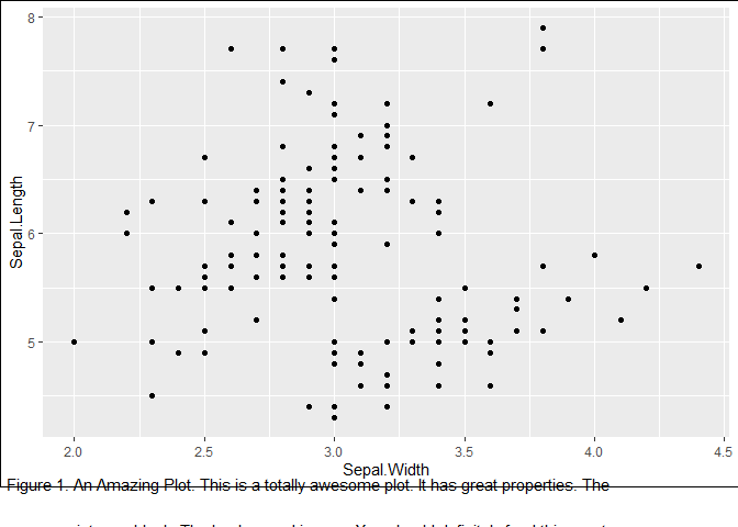

# notes - also good, but would like to have 
# plot box and figure_legend box align 
# bottom of plot box and top of figure_legend box on top of each other

# also still need lower lineheight/space between lines


#PLOTRIX option - not much success
library(plotrix)

Created on 2020-02-06 by the reprex package (v0.3.0)
Save it as pdf, open it in Illustrater, Inkscape etc, do whatever you want. Done!
Even though I also try to finish the plots as far as possible sometimes the last bits can take ages or aren't even possible. For example do you have an idea how you can put "Figure X" in bold but not the other text?
Especially in this case where you probably don't want to repeat this steps multiple times, but instead spend a lot of efforts to shine with this single (or few) figures.

2 Likes

In the spirit of @Matthias' answer, even Tufte finishes his graphics in Illustrator (not sure of what he's using now).

In theory, what you seek is possible, but I haven't been able to implement it tonight.

  1. Create a base object with a more visible border by upping to size = 2.5 for the data graph layer.
  2. Create an annotation layer for the legend with a similar visible border
  3. Glue the two globs together.

Sounds easy, doesn't it? (Nothing is impossible for the person who doesn't have to do it themselves.)

1 Like

The bold / not bold and selective italics issues can be handled with the ggtext package from Claus Wilke, found here: https://github.com/wilkelab/ggtext. I might have to ask Claus, who I rate above Tufte, and who has probably written multiple grants.

1 Like

While trying to access the ggtext package,
I am getting odd errors.
I can not install this one, or jpeg, or grid text.
But I can install other packages, like tidyverse and tidymodels.
Any ideas?
Error stream below...

remotes::install_github('wilkelab/ggtext')
Downloading GitHub repo wilkelab/ggtext@master
These packages have more recent versions available.
Which would you like to update?

1: All
2: CRAN packages only
3: None
4: ggplot2 (3.2.1 -> 6207d2f8d...) [GitHub]

Enter one or more numbers, or an empty line to skip updates:
1
ggplot2 (3.2.1 -> 6207d2f8d...) [GitHub]
gridtext (NA -> 0.1.0 ) [CRAN]
jpeg (NA -> 0.1-8.1 ) [CRAN]
Installing 2 packages: gridtext, jpeg
Error: Failed to install 'ggtext' from GitHub:
(converted from warning) unable to access index for repository https://cran.rstudio.com/bin/macosx/el-capitan/contrib/3.6:
cannot open URL 'https://cran.rstudio.com/bin/macosx/el-capitan/contrib/3.6/PACKAGES'

Ah, the wonderful wacky world of R on MAC OS!

More recent packages: I usually pick option 2, because not all packages are plug and play, some require compilation from source, which sometimes works and sometimes doesn't due to Apple's non-standard clang. Fortunately Saint Simon Urbanek on the R Core Development Team does the deep dive necessary to fix it and produces binaries. You can check CRAN under Packages to check whether it's available to install with update.packages().

If a package is on CRAN, but a later version is on github, you can run into the compilation problem and it may well contain features that you don't need yet.

I ran across the

unable to access index for repository https://cran.rstudio.com/bin/macosx/el-capitan/contrib/3.6:
cannot open URL 'https://cran.rstudio.com/bin/macosx/el-capitan/contrib/3.6/PACKAGES'

which indicates that their mirror is down. The answer is to pick another repository. I'm not sure where you are, so see the Mirrors link on CRAN.

install.packages(PACKAGE_NAME, repos='http://cran.rstudio.com/)
1 Like

Awesome package, is bookmarked, I will definitely need it at some point! :slightly_smiling_face:

1 Like

Thanks - I struggled with this a bit, but this document helped explain installing from tar to Mac http://www.ryantmoore.org/files/ht/htrtargz.pdf
Leaving this here in case someone finds this helpful for installing troublesome packages on Mac from binaries.

1 Like

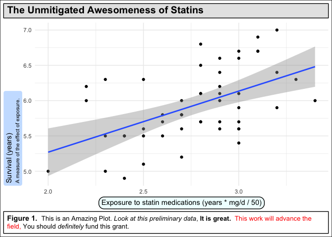
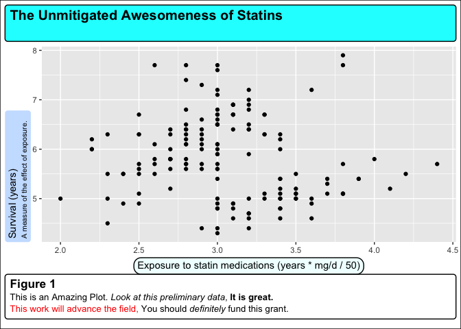
OK, I have a decent working version with ggtext.
It's mock data, but it is something.

library(tidyverse)
library(ggtext)

p <- iris %>% 
  ggplot() +
  aes(x= Sepal.Width, y = Sepal.Length) +
  geom_point()+
  theme(plot.background = element_rect(color='black'))

p + labs(
  title = "<b>The Unmitigated Awesomeness of Statins</b><br>",
  caption = "<b>Figure 1</b><br>
    <span style = 'font-size:10pt'>This is an Amazing Plot. *Look at this 
    preliminary data*, **It is great.**  
    <span style = 'color:red;'>This work will advance the field,</span> 
    You should *definitely* fund this grant.</span>",
  x = "Exposure to statin medications (years * mg/d / 50)",
  y = "Survival (years)<br><span style = 'font-size:8pt'>A measure of
    the effect of exposure.</span>"
) +
  theme(
    plot.title.position = "plot",
    plot.title = element_textbox_simple(
      size = 15,
      lineheight = 1,
      padding = margin(5.5, 5.5, 5.5, 5.5),
      margin = margin(0, 0, 5.5, 0),
      linetype = 1,
      fill = 'cyan1'
    ),
    plot.caption.position = "plot",
    plot.caption = element_textbox_simple(
      size = 13,
      lineheight = 1,
      padding = margin(5.5, 5.5, 5.5, 5.5),
      margin = margin(0, 0, 5.5, 0),
      linetype = 1
    ),
    axis.title.x = element_textbox_simple(
      width = NULL,
      padding = margin(4, 4, 4, 4),
      margin = margin(4, 0, 0, 0),
      linetype = 1,
      r = grid::unit(8, "pt"),
      fill = "azure1"
    ),
    axis.title.y = element_textbox_simple(
      hjust = 0,
      orientation = "left-rotated",
      minwidth = unit(1, "in"),
      maxwidth = unit(2, "in"),
      padding = margin(4, 4, 2, 4),
      margin = margin(0, 0, 2, 0),
      fill = "lightsteelblue1"
    )
  )

Created on 2020-02-08 by the reprex package (v0.3.0)

1 Like

This is quite close (except for the silly colors) to what I want.
The one thing I would like to change (because space limitations are tight) is to reduce the amount of space between the plot/caption and the background element.rect(). Is that a margins or padding issue?
Any suggestions on how to make the element rect tighter around the graphic elements?
thanks for any ideas,
Peter

I ended up downloading the tar file and putting it on my Mac desktop,

then used

install.packages('~/Desktop/jpeg_0.1-8.1.tar', repos = NULL, type ="source"

in the Rstudio console to install.

Then library(jpeg)

And then I could install ggtext.

1 Like

If you drop the oval border on the light blue, you can add \ns to get some more whitespace

Hey, way to go! For the benefit of those to come, please mark this as the solution (no false modesty!) the for the benefit of those to follow.

FAQ: How do I mark a solution?)

OK, for today's purposes, I will call this version the solution.

library(tidyverse)
library(ggtext)

p <- iris %>%
  filter(Species == 'versicolor') %>% 
  ggplot() +
  aes(x= Sepal.Width, y = Sepal.Length) +
  geom_point()+
  theme_minimal() +
  geom_smooth(method = 'lm') +
  theme(plot.background = element_rect(color='black')) 


p + labs(
  title = "<b>The Unmitigated Awesomeness of Statins</b>",
  caption = "<b>Figure 1.</b>
    <span style = 'font-size:10pt'>This is an Amazing Plot. *Look at this
    preliminary data*, **It is great.**
    <span style = 'color:red;'>This work will advance the field,</span>
    You should *definitely* fund this grant.</span>",
  x = "Exposure to statin medications (years * mg/d / 50)",
  y = "Survival (years)<br><span style = 'font-size:8pt'>A measure of
    the effect of exposure.</span>"
) +
  theme(
    plot.title.position = "plot",
    plot.title = element_textbox_simple(
      size = 15,
      lineheight = 1,
      padding = margin(4, 5.5, 4, 5.5), #padding inside the box, (trouble)
      margin = margin(0, 0, 7, 0), #margins outside the box, t,r,b,l
      linetype = 1,
      r = grid::unit(0, "pt"),
      fill = 'gray90'
    ),
    plot.caption.position = "plot",
    plot.caption = element_textbox_simple(
      size = 11,
      lineheight = 1.1,
      padding = margin(5.5, 5.5, 5.5, 5.5),
      margin = margin(0, 0, 0, 0),
      r = grid::unit(0, "pt"),
      linetype = 1
    ),
    axis.title.x = element_textbox_simple(
      width = NULL,
      padding = margin(4, 4, 4, 4),
      margin = margin(4, 0, 4, 0),
      linetype = 1,
      r = grid::unit(8, "pt"),
      fill = "azure1"
    ),
    axis.title.y = element_textbox_simple(
      hjust = 0,
      orientation = "left-rotated",
      minwidth = unit(1, "in"),
      maxwidth = unit(2, "in"),
      padding = margin(4, 4, 2, 4),
      margin = margin(0, 0, 2, 0),
      fill = "lightsteelblue1"
    )
  )
#> `geom_smooth()` using formula 'y ~ x'

Created on 2020-02-09 by the reprex package (v0.3.0)

1 Like

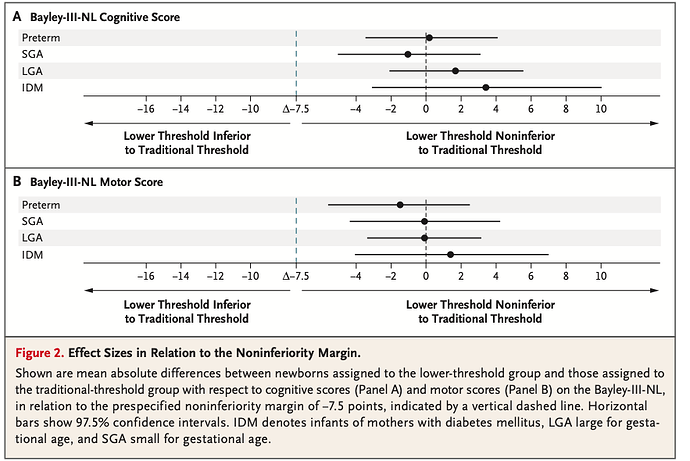
In a future state, I would like to make the standard multipanel plot seen in clinical research, with tags for figure panels A, B, etc., and a single text box figure legend for the figure at the bottom, as seen in a typical example here.
Ideally, one could make a multipanel plot with surrounding boxes and tags at top left (patchwork or cowplot or gridExtra), and a unifying figure legend in a text box with ggtext.
Any suggestions for this holy grail appreciated.

Again, this is from a guy who doesn't have to do it himself.

  1. The two-box solution should be extendable to three.
  2. The zero and \Delta -7.5 can be done by vline
  3. The A & B captions should be doable with ggtitle()
  4. The arrow legends might require yet another box.
  5. I'm guessing that there's a way to do the plots
  6. I'll wager the graybars have to be done postprocessing.

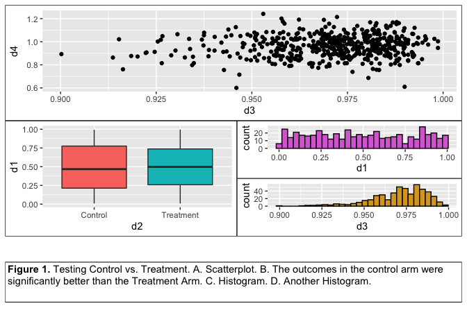
Getting closer
But still an odd space between plots and figure legend below

# Library calls
library(tidyverse)
library(grid)
library(gridtext)
library(ggtext)
library(patchwork)

# make dummy figures
d1 <- runif(500)
d2 <- rep(c("Treatment","Control"),each=250)
d3 <- rbeta(500,shape1=100,shape2=3)
d4 <- d3 + rnorm(500,mean=0,sd=0.1)
plotData <- data.frame(d1,d2,d3,d4)
str(plotData)
#> 'data.frame':    500 obs. of  4 variables:
#>  $ d1: num  0.0177 0.2228 0.5643 0.4036 0.329 ...
#>  $ d2: Factor w/ 2 levels "Control","Treatment": 2 2 2 2 2 2 2 2 2 2 ...
#>  $ d3: num  0.986 0.965 0.983 0.979 0.99 ...
#>  $ d4: num  0.876 0.816 1.066 0.95 0.982 ...

p1 <- ggplot(data=plotData) + geom_point(aes(x=d3, y=d4)) +
  theme(plot.background = element_rect(color='black'))
p2 <- ggplot(data=plotData) + geom_boxplot(aes(x=d2,y=d1,fill=d2))+
  theme(legend.position="none") +
  theme(plot.background = element_rect(color='black'))
p3 <- ggplot(data=plotData) +
  geom_histogram(aes(x=d1, color=I("black"),fill=I("orchid"))) +
  theme(plot.background = element_rect(color='black'))
p4 <- ggplot(data=plotData) +
  geom_histogram(aes(x=d3, color=I("black"),fill=I("goldenrod"))) +
  theme(plot.background = element_rect(color='black'))


fig_legend <- textbox_grob(
  "**Figure 1.**  Testing Control vs. Treatment.   A. Scatterplot. 
  B. The outcomes in the control arm were significantly better than 
  the Treatment Arm. C. Histogram. D. Another Histogram.",
  gp = gpar(fontsize = 11),
  box_gp = gpar(col = "black",   linetype = 1),
  padding = unit(c(3, 3, 3, 3), "pt"),
  margin = unit(c(0,0,0,0), "pt"),
  height = unit(0.6, "in"),
  width = unit(1, "npc"),
  #x = unit(0.5, "npc"), y = unit(0.7, "npc"),
  r = unit(0, "pt")
)
  

p1 + {
  p2 + {
    p3 +
      p4 +
      plot_layout(ncol=1)
  }
} + fig_legend +
  plot_layout(ncol=1)
#> `stat_bin()` using `bins = 30`. Pick better value with `binwidth`.

Created on 2020-02-09 by the reprex package (v0.3.0)

1 Like

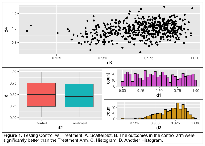
Better version with help from COW

SO discussion

note that the problem with the 'getting closer' version was that each row has (by default) equal height - so the figure legend was floating in an overly large vertical space.

Turn out that plot_annotation was designed for this purpose - handles this better.
Does need a tweak for L and R margins, which are inherited (+5/5) from plot above - therefore -5.5 for each L and R margin of the annotation.

# Library calls
library(tidyverse)
library(ggtext)
library(patchwork)

# make dummy figures
d1 <- runif(500)
d2 <- rep(c("Treatment","Control"), each=250)
d3 <- rbeta(500, shape1=100, shape2=3)
d4 <- d3 + rnorm(500, mean=0, sd=0.1)
plotData <- data.frame(d1, d2, d3, d4)

p1 <- ggplot(data=plotData) + geom_point(aes(x=d3, y=d4)) +
  theme(plot.background = element_rect(color='black'))
p2 <- ggplot(data=plotData) + geom_boxplot(aes(x=d2,y=d1,fill=d2))+
  theme(legend.position="none") +
  theme(plot.background = element_rect(color='black'))
p3 <- ggplot(data=plotData) +
  geom_histogram(aes(x=d1, color=I("black"),fill=I("orchid"))) +
  theme(plot.background = element_rect(color='black'))
p4 <- ggplot(data=plotData) +
  geom_histogram(aes(x=d3, color=I("black"),fill=I("goldenrod"))) +
  theme(plot.background = element_rect(color='black'))

fig_legend <- plot_annotation(
  caption = "**Figure 1.**  Testing Control vs. Treatment.   A. Scatterplot. 
  B. The outcomes in the control arm were significantly better than 
  the Treatment Arm. C. Histogram. D. Another Histogram.",
  theme = theme(
    plot.caption = element_textbox_simple(
      size = 11,
      box.colour = "black",
      linetype = 1,
      padding = unit(c(3, 3, 3, 3), "pt"),
      margin = unit(c(0, -5.5, 0, -5.5), "pt"), #note negative left and right margins because inherits margins from plots
      r = unit(0, "pt")
    )
  )
)


p1 + {
  p2 + {
    p3 +
      p4 +
      plot_layout(ncol=1)
  }
} + fig_legend +
  plot_layout(ncol=1)
#> `stat_bin()` using `bins = 30`. Pick better value with `binwidth`.

Created on 2020-02-09 by the reprex package (v0.3.0)

2 Likes

This topic was automatically closed 7 days after the last reply. New replies are no longer allowed.