Piecewise quantile linear regression with "quantreg" and "segmented" package

[Dteruel_94]

Hello, I am looking for a way to obtain the piecewise quantile linear regression with R. I have been able to compute the Quantile regression with the package quantreg . However, I don't want just 1 unique slope but want to check for breakpoints in my fit. I have seen that the segmented package can do so. While it works good if the fit is carried out with lm or glm (as shown below in an example), it doesn't manage to work for quantile.

On the segmented package info I have read that there is a segmented.default which can be used for specific regression models, such as Quantiles. However, when I apply it for my quantile outcome it gives me the following errors:

Error in diag(vv) : invalid 'nrow' value (too large or NA) In addition: Warning message: cannot compute the covariance matrix.

I have created an example with the mtcars data so you can see the errors that I get.

library(quantreg)
library(segmented)

data(mtcars)

out.rq <- rq(mpg ~ wt, data= mtcars)
out.lm <- lm(mpg ~ wt, data= mtcars)

# Plotting the results
plot(mpg ~ wt, data = mtcars, pch = 1, main = "mpg ~ wt") 
abline(out.lm, col = "red", lty = 2)
abline(out.rq, col = "blue", lty = 2)
legend("topright", legend = c("linear", "quantile"), col = c("red", "blue"), lty = 2)

#Generating segmented LM
o <- segmented(out.lm, seg.Z= ~wt, npsi=2, control=seg.control(display=FALSE))  
plot(o, lwd=2, col=2:6, main="Segmented regression", res=FALSE) #lwd: line width #col: from 2 to 6 #RES: show datapoints

#Generating segmented Quantile
o.quantile <- segmented.default(out.rq, seg.Z= ~wt, npsi=2, control=seg.control(fn.obj=out.rq$rho))   

From what I have seen, it has to do with the calculation of the vcov but I have not been able to figure out how to fix it.
Thanks in advance

[technocrat]

Hi, and welcome!

Thanks for the reprex!

The problematic line is

 o.quantile <- segmented.default(out.rq, seg.Z= ~wt, npsi=2, control=seg.control(fn.obj=out.rq$rho))

Error in diag(vv) : invalid 'nrow' value (too large or NA)
In addition: Warning messages:
1: max number of iterations (1) attained 
2: In rq.fit.br(x, y, tau = tau, ...) : Solution may be nonunique
3: cannot compute the covariance matrix 

There are two flavors here:

1. The error, which is a show stopper indicating the reason that segmented.default failed to produce o.quantile.
2. The warning put the user on notice that the fitted model's properties derived from the call on the underlying data:

• Would have limited successful completion to a single iteration
• May have produced two or more solutions
• Would not have returned a covariance matrix

The help(segmented) page has useful detail on models other than lm and glm

Since version 0.5-0.0 the default method segmented.default has been added to estimate segmented relationships in general (besides "lm" and "glm" fits) regression models, such as Cox regression or quantile regression (for a single percentile). The objective function to be minimized is the (minus) value extracted by the logLik function or it may be passed on via the fn.obj argument in seg.control. See example below. While the default method is expected to work with any regression fit (where the usual coef(), update(), and logLik() returns appropriate results), it is not recommended for "lm" or "glm" fits (as segmented.default is slower than the specific methods segmented.lm and segmented.glm), although final results are the same. However the object returned by segmented.default is not of class "segmented", as currently the segmented methods are not guaranteed to work for ‘generic’ (i.e., besides "lm" and "glm") regression fits. The user could try each "segmented" method on the returned object by calling it explicitly (e.g. via plot.segmented() or confint.segmented()).

That points to looking at the out.rq object

summary(out.rq)
Call: rq(formula = mpg ~ wt, data = mtcars)

tau: [1] 0.5

Coefficients:
            coefficients lower bd upper bd
(Intercept) 34.23224     32.25029 39.74085
wt          -4.53947     -6.47553 -4.16390
Warning message:
In rq.fit.br(x, y, tau = tau, ci = TRUE, ...) : Solution may be nonunique
> coef(out.rq)
(Intercept)          wt 
  34.232237   -4.539474 

update(out.rq)
Call:
rq(formula = mpg ~ wt, data = mtcars)

Coefficients:
(Intercept)          wt 
  34.232237   -4.539474 

Degrees of freedom: 32 total; 30 residual

logLik(out.rq)
'log Lik.' -81.13212 (df=2)

Compare this to

library(quantreg)
#> Loading required package: SparseM
#> 
#> Attaching package: 'SparseM'
#> The following object is masked from 'package:base':
#> 
#>     backsolve
library(segmented)

data(engel)
attach(engel)

# Example of plotting of coefficients and their confidence bands
# (from help(rq))

example_rq <- rq(foodexp~income,tau = 1:49/50,data=engel)
coef(example_rq)
#>               tau= 0.02   tau= 0.04   tau= 0.06   tau= 0.08   tau= 0.10
#> (Intercept) 108.6049876 111.9619666 121.2614673 115.5693385 110.1415742
#> income        0.3466438   0.3459667   0.3546998   0.3741786   0.4017658
#>               tau= 0.12   tau= 0.14   tau= 0.16   tau= 0.18   tau= 0.20
#> (Intercept) 113.1731206 118.3558209 107.2653239 106.0644961 102.3138823
#> income        0.4034456   0.4076138   0.4303873   0.4377145   0.4468995
#>               tau= 0.22  tau= 0.24  tau= 0.26  tau= 0.28 tau= 0.30   tau= 0.32
#> (Intercept) 100.7499983 93.0013627 93.0258079 94.3928676  99.11058 104.5752061
#> income        0.4584563  0.4753133  0.4785695  0.4831288   0.48124   0.4806967
#>               tau= 0.34  tau= 0.36   tau= 0.38   tau= 0.40  tau= 0.42 tau= 0.44
#> (Intercept) 104.8746113 109.264465 111.2591182 101.9598824 96.8304800 87.352278
#> income        0.4883315   0.487097   0.4882341   0.5098965  0.5202734  0.538949
#>              tau= 0.46  tau= 0.48  tau= 0.50  tau= 0.52  tau= 0.54 tau= 0.56
#> (Intercept) 84.0313073 85.5779856 81.4822474 89.5718087 95.5653415 89.869714
#> income       0.5512162  0.5505803  0.5601806  0.5565181  0.5538046  0.565769
#>              tau= 0.58  tau= 0.60  tau= 0.62  tau= 0.64  tau= 0.66  tau= 0.68
#> (Intercept) 83.6047146 79.7022726 82.4143976 73.0744013 73.6645497 76.9492185
#> income       0.5783635  0.5858492  0.5866155  0.6051067  0.6095186  0.6098483
#>             tau= 0.70  tau= 0.72  tau= 0.74  tau= 0.76  tau= 0.78  tau= 0.80
#> (Intercept) 79.283617 63.0579071 67.3117885 54.3632674 52.0872017 58.0066635
#> income       0.608851  0.6368253  0.6373555  0.6540243  0.6620919  0.6595106
#>              tau= 0.82  tau= 0.84  tau= 0.86  tau= 0.88  tau= 0.90  tau= 0.92
#> (Intercept) 59.8850860 55.3874764 58.3310147 75.6104227 67.3508721 63.3247451
#> income       0.6601063  0.6710072  0.6762091  0.6661093  0.6862995  0.6977259
#>              tau= 0.94  tau= 0.96  tau= 0.98
#> (Intercept) 68.7959047 59.2255920 84.1675685
#> income       0.7007916  0.7198025  0.7096649
update(example_rq)
#> Call:
#> rq(formula = foodexp ~ income, tau = 1:49/50, data = engel)
#> 
#> Coefficients:
#>               tau= 0.02   tau= 0.04   tau= 0.06   tau= 0.08   tau= 0.10
#> (Intercept) 108.6049876 111.9619666 121.2614673 115.5693385 110.1415742
#> income        0.3466438   0.3459667   0.3546998   0.3741786   0.4017658
#>               tau= 0.12   tau= 0.14   tau= 0.16   tau= 0.18   tau= 0.20
#> (Intercept) 113.1731206 118.3558209 107.2653239 106.0644961 102.3138823
#> income        0.4034456   0.4076138   0.4303873   0.4377145   0.4468995
#>               tau= 0.22  tau= 0.24  tau= 0.26  tau= 0.28 tau= 0.30   tau= 0.32
#> (Intercept) 100.7499983 93.0013627 93.0258079 94.3928676  99.11058 104.5752061
#> income        0.4584563  0.4753133  0.4785695  0.4831288   0.48124   0.4806967
#>               tau= 0.34  tau= 0.36   tau= 0.38   tau= 0.40  tau= 0.42 tau= 0.44
#> (Intercept) 104.8746113 109.264465 111.2591182 101.9598824 96.8304800 87.352278
#> income        0.4883315   0.487097   0.4882341   0.5098965  0.5202734  0.538949
#>              tau= 0.46  tau= 0.48  tau= 0.50  tau= 0.52  tau= 0.54 tau= 0.56
#> (Intercept) 84.0313073 85.5779856 81.4822474 89.5718087 95.5653415 89.869714
#> income       0.5512162  0.5505803  0.5601806  0.5565181  0.5538046  0.565769
#>              tau= 0.58  tau= 0.60  tau= 0.62  tau= 0.64  tau= 0.66  tau= 0.68
#> (Intercept) 83.6047146 79.7022726 82.4143976 73.0744013 73.6645497 76.9492185
#> income       0.5783635  0.5858492  0.5866155  0.6051067  0.6095186  0.6098483
#>             tau= 0.70  tau= 0.72  tau= 0.74  tau= 0.76  tau= 0.78  tau= 0.80
#> (Intercept) 79.283617 63.0579071 67.3117885 54.3632674 52.0872017 58.0066635
#> income       0.608851  0.6368253  0.6373555  0.6540243  0.6620919  0.6595106
#>              tau= 0.82  tau= 0.84  tau= 0.86  tau= 0.88  tau= 0.90  tau= 0.92
#> (Intercept) 59.8850860 55.3874764 58.3310147 75.6104227 67.3508721 63.3247451
#> income       0.6601063  0.6710072  0.6762091  0.6661093  0.6862995  0.6977259
#>              tau= 0.94  tau= 0.96  tau= 0.98
#> (Intercept) 68.7959047 59.2255920 84.1675685
#> income       0.7007916  0.7198025  0.7096649
#> 
#> Degrees of freedom: 235 total; 233 residual
logLik(example_rq)
#> 'log Lik.' -1492.796, -1477.893, -1471.161, -1465.414, -1459.198, -1453.010, -1448.369, -1443.113, -1439.291, -1435.883, -1433.075, -1430.201, -1427.488, -1425.055, -1423.283, -1421.885, -1420.634, -1419.524, -1418.784, -1418.006, -1417.122, -1415.842, -1413.964, -1412.599, -1411.630, -1410.804, -1410.206, -1409.542, -1408.870, -1408.359, -1408.271, -1408.245, -1408.238, -1408.086, -1408.604, -1409.221, -1409.456, -1409.944, -1410.668, -1412.032, -1414.064, -1416.784, -1420.184, -1424.081, -1428.220, -1431.968, -1437.940, -1447.796, -1468.227 (df=2)
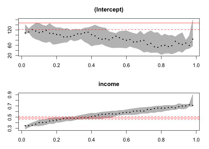
plot(summary(rq(foodexp~income,tau = 1:49/50,data=engel)))
#> Warning in rq.fit.br(x, y, tau = tau, ci = TRUE, ...): Solution may be nonunique

#> Warning in rq.fit.br(x, y, tau = tau, ci = TRUE, ...): Solution may be nonunique

#> Warning in rq.fit.br(x, y, tau = tau, ci = TRUE, ...): Solution may be nonunique

#> Warning in rq.fit.br(x, y, tau = tau, ci = TRUE, ...): Solution may be nonunique

^{Created on 2020-04-06 by the reprex package (v0.3.0)}

The differences to me, based solely on the documentation suggest trying different rq object to see if the return values are similar to the example and, if so, whether segmented.default will return its expected value.

Again, for emphasis, I have not used rq before, so I'm approaching the question from a purely formal function signature basis.