PCA - how to include categorical variables like countries

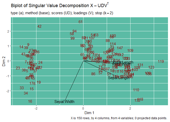
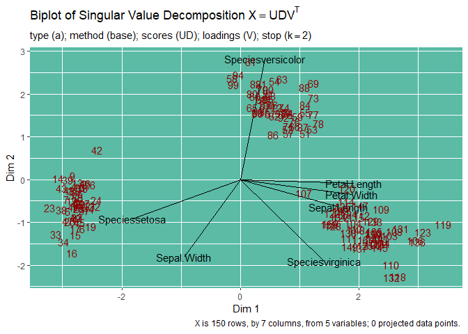
Hi. I am new in R. I was trying to figure out how to incorporate categorical variables in PCA. prcomp and ePCA only compute numeric variables. But I want to analyze the countries as well. any help, please?

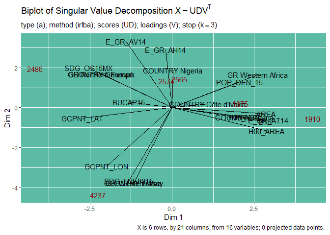
#dataset #592 obs. of 17 variables

head(UrbanAreaLog)
ID AREA GCPNT_LAT GCPNT_LON COUNTRY GR UC_NAME
1 2486 49 57.0410899168 9.92426287095 Denmark Northern Europe Aalborg
2 2574 96 5.10886858483 7.35086200977 Nigeria Western Africa Aba
3 1675 431 5.34956326151 -4.00269599617 Côte d'Ivoire Western Africa Abidjan
4 2565 337 9.06189891144 7.43349518867 Nigeria Western Africa Abuja
5 1910 846 5.62108507064 -0.215586874558 Ghana Western Africa Accra
6 4237 135 37.0034193536 35.2831339317 Turkey Western Asia Adana
H00_NBR H00_AREA B15 BUCAP15 E_GR_AV14 E_GR_AH14 E_GR_AT14 SDG_LUE9015
1 1 3.891820 3.333719 5.635509 -0.7241529 3.498985 3.890039 -0.8076205
2 1 4.418841 3.569795 3.390930 -1.1212652 3.019277 4.553592 -2.2733364
3 1 5.894403 5.441951 3.926418 -1.3018480 3.628108 6.056978 -1.3642453
4 1 4.718499 4.906370 4.534689 -1.0133702 4.246865 5.811337 -1.0336720
5 2 6.513230 6.204348 4.719880 -1.2254961 2.680334 6.732362 -1.4974861
6 1 4.836282 4.174412 4.478802 -1.4558008 2.454523 4.910071 6.3459896
SDG_OS15MX POP_DEN_15
1 4.212276 5.604330
2 4.143293 7.370860
3 3.837946 5.818301
4 4.092677 5.786284
5 3.725693 7.675128
6 3.948355 5.071417

pca method 1
UrbanArea_pca <- UrbanAreaLog %>%
filter(GR %in% c("Australia/New Zealand","Caribbean","Central America","Eastern Africa","Eastern Europe",
"Middle Africa","Northern Africa","Northern America","Northern Europe","South America",
"South-Central Asia","Southern Africa","Southern Europe","Western Africa","Western Asia",
"Western Europe")) %>%
dplyr::select(COUNTRY,UC_NAME,GR,ID,H00_AREA,B15,BUCAP15,E_GR_AV14,E_GR_AH14,E_GR_AT14,SDG_LUE9015,SDG_OS15MX,POP_DEN_15) %>%
unite("continent_country_city", c(COUNTRY,GR,UC_NAME,ID)) %>%
column_to_rownames("continent_country_city")

UrbanArea.pca2 <- prcomp(na.omit(UrbanArea_pca, scale=TRUE))

#the above script does work but it combines classes into one

pca method 2
UrbanF.pca <- epPCA(na.omit(UrbanAreaLog[-1:-8], graph=FALSE))

fviz_pca_ind(UrbanF.pca,
geom.ind = "point", # show points only (nbut not "text")
col.ind.sup = (UrbanAreaLog$UC_NAME), # color by groups
palette = c("rainbow"),
addEllipses = TRUE, # Concentration ellipses
legend.title = "Geographic Regions")

#this method 2 does not show classes by groups

Hi Kris

I've used one-hot encoding to good effect.

For illustration, here is the usual biplot of the four numerical variables in iris.

Now one-hot encode the categorical variables. e.g. Species in the iris dataset has three factor levels: setosa, versicolor and virginica so the Species column expands to three binary columns treated as numeric.

#>   Sepal.Length Sepal.Width Petal.Length Petal.Width Speciessetosa
#> 1          5.1         3.5          1.4         0.2             1
#> 2          4.9         3.0          1.4         0.2             1
#> 3          4.7         3.2          1.3         0.2             1
#> 4          4.6         3.1          1.5         0.2             1
#> 5          5.0         3.6          1.4         0.2             1
#> 6          5.4         3.9          1.7         0.4             1
#>   Speciesversicolor Speciesvirginica
#> 1                 0                0
#> 2                 0                0
#> 3                 0                0
#> 4                 0                0
#> 5                 0                0
#> 6                 0                0

Here is the biplot of the one-hot expanded data set.

Created on 2019-07-22 by the reprex package (v0.3.0)

hi. thanks. I used the ff code for visualization:
g <- ggbiplot(mydata, obs.scale = 1, var.scale = 1,
groups = mydata.cities, ellipse = TRUE,
circle = TRUE)
g <- g + scale_color_discrete(name = '')
g <- g + theme(legend.direction = 'horizontal',
legend.position = 'top')

but i have this error:
Error in $<-.data.frame(*tmp*, "groups", value = c("Northern Europe", :
replacement has 592 rows, data has 463

Hi Kris

At this point we need access to some minimal data set and to your reproducible code. Try to make a reproducible example to post. The reprex package is a fantastic tool. Here is the FAQ: What's a reproducible example (`reprex`) and how do I do one?

I for one would like to see more of this and help this kind analysis.

From the head() snapshot of your data this is the best I can do to reconstruct a portion (six observation). Normally I'd want to just run something from your example and get a good chunk of data to work with and recreate your issue without having to put in this extra effort.

You could do something like this:

# your data encoded as a character string using `deparse()` and pasted in here.
x_ <- c(
    "structure(list(ID = c(2486L, 2574L, 1675L, 2565L, 1910L, 4237L",
    "), AREA = c(49L, 96L, 431L, 337L, 846L, 135L), GCPNT_LAT = c(57.0410899168, ",               
    "5.10886858483, 5.34956326151, 9.06189891144, 5.62108507064, 37.0034193536",
    "), GCPNT_LON = c(9.92426287095, 7.35086200977, -4.00269599617, ",                            
    "7.43349518867, -0.215586874558, 35.2831339317), COUNTRY = structure(c(2L, ",
    "4L, 1L, 4L, 3L, 5L), .Label = c(\" Côte d'Ivoire\", \" Denmark\", ",                        
    "\" Ghana\", \" Nigeria\", \" Turkey\"), class = \"factor\"), GR = structure(c(1L, ",
    "2L, 2L, 2L, 2L, 3L), .Label = c(\" Northern Europe\", \" Western Africa\", ",                
    "\" Western Asia\"), class = \"factor\"), UC_NAME = structure(1:6, .Label = c(\" Aalborg\", ",
    "\" Aba\", \" Abidjan\", \" Abuja\", \" Accra\", \" Adana\"), class = \"factor\"), ",         
    "    H00_NBR = c(1L, 1L, 1L, 1L, 2L, 1L), H00_AREA = c(3.89182, ",
    "    4.418841, 5.894403, 4.718499, 6.51323, 4.836282), B15 = c(3.333719, ",                   
    "    3.569795, 5.441951, 4.90637, 6.204348, 4.174412), BUCAP15 = c(5.635509, ",
    "    3.39093, 3.926418, 4.534689, 4.71988, 4.478802), E_GR_AV14 = c(-0.7241529, ",            
    "    -1.1212652, -1.301848, -1.0133702, -1.2254961, -1.4558008",
    "    ), E_GR_AH14 = c(3.498985, 3.019277, 3.628108, 4.246865, ",                              
    "    2.680334, 2.454523), E_GR_AT14 = c(3.890039, 4.553592, 6.056978, ",
    "    5.811337, 6.732362, 4.910071), SDG_LUE9015 = c(-0.8076205, ",                            
    "    -2.2733364, -1.3642453, -1.033672, -1.4974861, 6.3459896), ",
    "    SDG_OS15MX = c(4.212276, 4.143293, 3.837946, 4.092677, 3.725693, ",                      
    "    3.948355), POP_DEN_15 = c(5.60433, 7.37086, 5.818301, 5.786284, ",
    "    7.675128, 5.071417)), class = \"data.frame\", row.names = c(2486L, ",                    
    "2574L, 1675L, 2565L, 1910L, 4237L))"
)

# parse the string to get the data frame `x`
x <- eval(parse(text= x_))

# use the ID column as rownames
rownames(x) <- x$ID

# OK, this next bit won't be reproducible on your side, but you have to put in some 
# work to include your reproducible code here. e.g. I'd have to extract a minimal 
# working version of the code from my functions `T1` and `plot.T1`.

# If you get used to using `reprex` this becomes a breeze, a joy.

x[-1] %>% T1() %>% plot(type. = "a")

Here's what I'm trying to illustrate: this is an example of what you could get with one-hot encoding of your categorical variables, but of course this hardly shows it here with only six observations.

Is this the sort of thing you're looking for?

Created on 2019-07-23 by the reprex package (v0.3.0)

This topic was automatically closed 21 days after the last reply. New replies are no longer allowed.