Pareto Distribution

[hhu]

I wrote down the code for an inversion sampler to generate a sample of N = 1000 random numbers from the Pareto distribution with a = 2 and b = 3. Use the generated CNRG pseudo-random numbers.

Xo<-33475781
a<-3
c<-5
m<-1000
U <- numeric(length = m)
U[1]<-Xo
for(i in 2:m){
  U[i] <- (a*U[i-1]+c)%%m
}
inv<-function(U,A,b) {
  A/((U)^(1/b))
}
pareto<-inv(U,A=2,b=3)

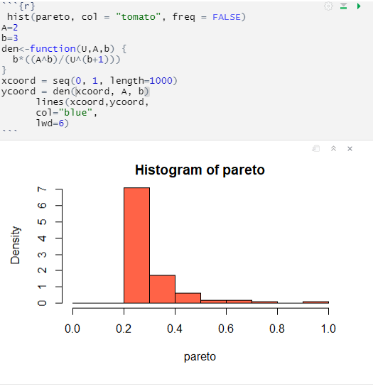
and then Draw a histogram for the generated sample and add a line with the true density of the Pareto(2, 3) distribution, but the density line doesn't show up on the graph.

 hist(pareto, col = "tomato", freq = FALSE)
A=2
b=3
den<-function(U,A,b) {
  b*((A^b)/(U^(b+1)))
}
xcoord = seq(0, 1, length=1000)
ycoord = den(xcoord, A, b)
      lines(xcoord,ycoord,
      col="blue",
      lwd=6)

if I change ycoord = den(U, A, b) instead,
then there's only a straight line in the bottom.

How can I fix the problem?
Thank you

[DavoWW]

Hi @hhu,
Welcome to the RStudio Community Forum.

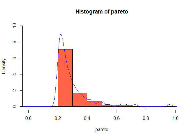
Looks like your density function is producing incorrect values which are way off the Y scale. Try using the built-in density() function:

# Generate distribution
Xo <- 33475781
a <- 3
c <- 5
m <- 1000
U <- numeric(length = m)
U[1] <- Xo
for(i in 2:m){
  U[i] <- (a*U[i-1]+c)%%m
}

inv <- function(U,A,b) {
  A/((U)^(1/b))
}
pareto <- inv(U, A=2, b=3)

# Home-made density function
A <- 2
b <- 3
den <- function(U, A, b) {
  b*((A^b)/(U^(b+1)))
}

xcoord <- seq(0, 1, length=1000)
ycoord <- den(xcoord, A, b)

# Large mismatch in Y scales
summary(pareto)
#>     Min.  1st Qu.   Median     Mean  3rd Qu.     Max. 
#> 0.006206 0.220227 0.251235 0.293390 0.314193 0.961500
summary(ycoord)      
#>    Min. 1st Qu.  Median    Mean 3rd Qu.    Max. 
#>   24.00   75.85  384.00     Inf 6144.19     Inf

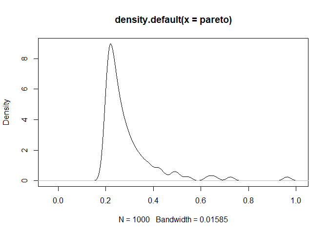
# Use built-in density function?
plot(density(pareto))

myden <- density(pareto)

hist(pareto, col = "tomato", freq = FALSE, ylim=c(0, 10))
lines(myden$x, myden$y, type="l", col="blue")

^{Created on 2021-08-05 by the reprex package (v2.0.0)}