Numerical Methods: Creation of a graph in which the function moves inwards the higher the parameter gamma

[Michael_DG]

Hi Posit Community,

I am doing numerical methods and I am struggling to produce the PNG file that is enclosed:

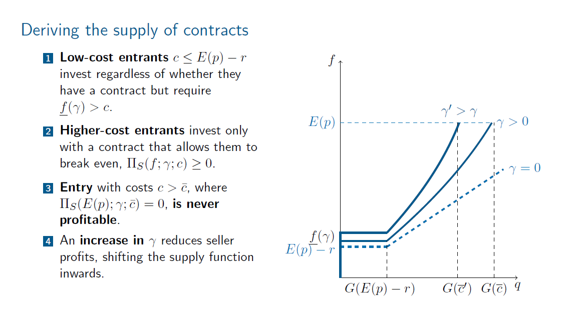
Below is my code using reprex(), in which I try to replicate this, but obtained a completely different graph:

# Required libraries
if (!require("pacman")) install.packages("pacman")
pacman::p_load(ggplot2, tidyverse, hrbrthemes, gridExtra, cubature, formattable, rootSolve, readr, pracma, here, fs, truncdist, xtable, reshape2, writexl)

# Define the necessary functions
compute_R_gamma <- function(f, gamma, r, alpha, beta) {
  # Handle boundary conditions
  if (f == 0 || gamma == 0) {
    return(0)
  }
  if (f == 1 && gamma == 1) {
    return(r)
  }
  
  # Compute the variance of p
  var_p <- (alpha * beta) / ((alpha + beta)^2 * (alpha + beta + 1))
  
  # Function to calculate the variance of the minimum of p and f
  var_tilde_p <- function(f, alpha, beta) {
    # Define the PDF of the Beta distribution
    beta_pdf <- function(p) dbeta(p, alpha, beta)
    
    # Define the CDF of the Beta distribution
    beta_cdf <- function(p) pbeta(p, alpha, beta)
    
    # First moment of tilde_p (E[tilde_p])
    first_moment <- integrate(function(p) {
      p * beta_pdf(p)
    }, lower = 0, upper = f)$value + f * (1 - beta_cdf(f))
    
    # Second moment of tilde_p (E[tilde_p^2])
    second_moment <- integrate(function(p) {
      p^2 * beta_pdf(p)
    }, lower = 0, upper = f)$value + f^2 * (1 - beta_cdf(f))
    
    # Variance of tilde_p
    second_moment - first_moment^2
  }
  
  # Compute the variance of tilde_p
  var_tilde_p_value <- var_tilde_p(f, alpha, beta)
  
  # Compute R_gamma(f, gamma)
  R_gamma_value <- r * gamma^2 * (var_tilde_p_value / var_p)
  
  return(R_gamma_value)
}

contract_market_profit <- function(f, gamma, c, r, alpha, beta) {
  term1 <- f * (1 - gamma * pbeta(f, alpha, beta))
  term2 <- gamma * integrate(function(p) p * dbeta(p, alpha, beta), lower = 0, upper = f)$value
  term3 <- compute_R_gamma(f, gamma, r, alpha, beta)
  return(term1 + term2 - term3 - c)
}

spot_market_profit <- function(c, mean_p, r) {
  return(mean_p - r - c)
}

# Function to find f_underline by solving the equality of profits
find_f_underline <- function(c, gamma, r, alpha, beta, mean_p) {
  # Define the function representing the difference in profits
  profit_difference <- function(f) {
    contract_market_profit(f, gamma, c, r, alpha, beta) - spot_market_profit(c, mean_p, r)
  }
  
  # Use uniroot to find the root of the profit difference function
  result <- tryCatch(
    uniroot(profit_difference, lower = mean_p - r, upper = mean_p)$root,
    error = function(e) NA
  )
  
  # Ensure the found f_underline is greater than or equal to E(p) - r
  if (!is.na(result) && result >= (mean_p - r)) {
    return(result)
  } else {
    return(NA)
  }
}

# Calculate the break-even investment cost c_break_even for a given gamma
find_c_break_even <- function(gamma, r, alpha, beta, mean_p) {
  tryCatch(
    uniroot(
      function(c) contract_market_profit(mean_p, gamma, c, r, alpha, beta),
      lower = 0, upper = 1  # Search interval for c, this could be adjusted depending on context
    )$root,
    error = function(e) NA
  )
}

# Calculate the highest investment cost c_bar(gamma) for which entry might be profitable
find_c_bar <- function(gamma, r, alpha, beta, mean_p) {
  # The highest investment cost such that the seller breaks even at f = E(p)
  find_c_break_even(gamma, r, alpha, beta, mean_p)
}

# Categorize entrants based on their costs
categorize_entry <- function(c, gamma, r, alpha, beta, mean_p) {
  # Calculate key thresholds
  f_lower_bound <- mean_p - r  # E(p) - r
  c_bar <- find_c_bar(gamma, r, alpha, beta, mean_p)
  
  # Check conditions for categorization
  if (c > c_bar || is.na(c_bar)) {
    return("No Entry (c > c_bar)")
  } else if (c <= f_lower_bound) {
    return("Low-Cost Entrant (c <= E(p) - r)")
  } else {
    return("Higher-Cost Entrant (c > E(p) - r)")
  }
}

# Initialize parameters
c_values <- seq(0, 1, by = 0.05)      # Example c values
gamma_values <- seq(0, 1, by = 0.1)  # Example gamma values
alpha <- 4                            # Alpha parameter of Beta distribution
beta <- 2                             # Beta parameter of Beta distribution
r <- 0.4                              # Risk premium
mean_p <- 0.6                         # E(p)

# Generate results for all combinations of gamma and c
entry_results <- data.frame()

for (gamma in gamma_values) {
  c_bar <- find_c_bar(gamma, r, alpha, beta, mean_p)  # Compute c_bar
  
  if (!is.na(c_bar)) {
    for (c in c_values) {
      # Compute specific f(gamma) using find_f_underline
      f_specific <- find_f_underline(c, gamma, r, alpha, beta, mean_p)
      
      # Compute E(p) - r (lower bound for low-cost entrants)
      lower_f_gamma <- mean_p - r
      
      # Compute profits in both markets
      profit_spot <- spot_market_profit(c, mean_p, r)
      profit_contract <- if (!is.na(f_specific)) {
        contract_market_profit(f_specific, gamma, c, r, alpha, beta)
      } else {
        NA
      }
      
      # Entrant Type Logic (with explicit NA checks)
      if (c > c_bar) {
        entrant_type <- "No Entry (c > c_bar)"
      } else if (c <= lower_f_gamma && !is.na(f_specific) && f_specific > c) {
        entrant_type <- "Low-Cost Entrant (c <= E(p) - r)"
      } else if (!is.na(profit_contract) && profit_contract >= c) {
        entrant_type <- "Higher-Cost Entrant (c > E(p) - r)"
      } else if (lower_f_gamma < c) {
        entrant_type <- "f(gamma) < c"
      } else {
        entrant_type <- "Undefined"
      }
      
      # Store results in entry_results
      entry_results <- rbind(
        entry_results,
        data.frame(
          gamma = gamma,
          c = c,
          c_bar = c_bar,
          f_specific = f_specific,
          lower_f_gamma = lower_f_gamma,
          profit_spot = profit_spot,
          profit_contract = profit_contract,
          profit_difference = profit_contract - profit_spot,
          c_bar_normalized = pmin(c / c_bar, 1),
          entrant_type = entrant_type
        )
      )
    }
  }
}

# Plot the results
ggplot(entry_results, aes(x = c_bar_normalized, y = f_specific, color = factor(gamma))) +
  geom_line(linewidth = 1) +
  geom_point(size = 2, alpha = 0.7) +
  labs(
    title = "Cumulative Supply G(c) vs Contract Prices f(gamma)",
    x = "Cumulative Supply G(c)",
    y = "Contract Price f(gamma)",
    color = "Gamma (Proportion of Opportunistic Buyers)"
  ) +
  theme_minimal() +
  scale_color_brewer(palette = "Dark2")

# Print the results
print(entry_results)

and the graph obtained does not look at all at the one shown above.

Any ideas how I can obtain more or less the first figure shown above, please? Thank you so much.

Michael