Multiple Vector Plot + line colours and marking

[NathanS]

Hi there, I am trying to plot the data below, but I am struggling to figure out how to plot multiple vectors with different lengths. Since they are different lengths, I wasn't able to use a data frame and instead, I have tried to put it in list form and based on other forums I tried to use mapply but I am now struggling to figure out how to manually (not arbitrarily) set individual colors for each line in the plot and to put dots on the lines where they correspond to a data point (for example a = 0.95). Any advice on how to maybe more efficiently but also more intuitively solve this problem is welcome.

xstar=0.85
x1 =  c(0.8262858, 0.9102857, 0.9032932, 0.8994474, 0.8994474)
x2 =  c(0.8151768, 0.9053250, 0.8994474, 0.8975376, 0.8975376)
a =  c(0.3000000, 0.8151768, 0.8151768, 0.8151768, 0.8151768, 0.8151768)
b = c(0.9500000, 0.9500000, 0.9102857, 0.8994474, 0.8994474, 0.8994474)


biaspl = list(x1 = c(x1), x2 = c(x2), a = c(a), b = c(b))


plot(unlist(biaspl), type = "l", main = "Evolution of Legal Threshold and Effort Levels", xlim = c(1,length(period)), ylim = (0:1),xlab = expression("Time Period (t)"),ylab = expression("Threshold/Effort Level"))
  axis(side=2,seq(0,1,0.1))
  axis(side=1,seq(0,5,1))
  abline(h = xstar, col=("yellow"), lwd=2, lty=1)
  mapply(lines, biaspl, col="blue")
  legend("bottomright", c("x1","x2","a","b"), fill = c("blue","red","green","green"))

[technocrat]

This calls out for building up a plot through ggplot2, which I'm attempting. Based only on the legending, I'm guessing this is a time series of four variables, two of which are observed at 5 points in time and two of which are observed at 6.

It also looks like all four variables are bound in 0 and 1.

The desired chart has an x-axis of sequential periods and a y-axis of values between 0 and 1. The aesthetics are points of each variable and the line connecting them. The variables should be distinguished by some combination of color, line width, line style and point style. The whole should have the indicated title and legend.

Have I got that right?

[NathanS]

Yes that is exactly right!

[technocrat]

Then you write great code! Let me chew on this for a bit and will get back to you.

[technocrat]

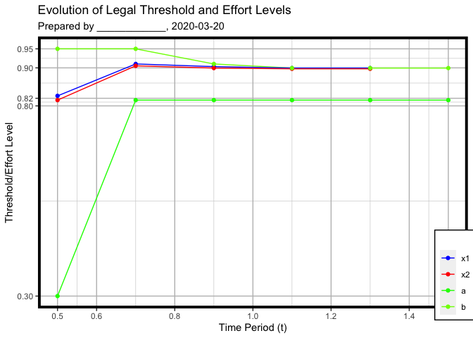
Here is one out of infinitely ways of doing this in ggplot2 Tweaking is required to get the legend box placement entirely to fit on any given plot device.

suppressPackageStartupMessages(library())
suppressPackageStartupMessages(library(ggplot2))
suppressPackageStartupMessages(library(magrittr))
suppressPackageStartupMessages(library(scales))
suppressPackageStartupMessages(library(tidyr))

# create varible for x-axis
timed <- seq(from = 0.5, to = 1.5, by = 0.2)
# variables from the last post
x1 =  c(0.8262858, 0.9102857, 0.9032932, 0.8994474, 0.8994474)
x2 =  c(0.8151768, 0.9053250, 0.8994474, 0.8975376, 0.8975376)
a =  c(0.3000000, 0.8151768, 0.8151768, 0.8151768, 0.8151768, 0.8151768)
b = c(0.9500000, 0.9500000, 0.9102857, 0.8994474, 0.8994474, 0.8994474)

# create a data frame, ignoring warning about unequal lengths
# x1 and x2 will recycle first value to fill in the missing values
# timed, instead of time, to avoid namespace collision
as.data.frame(cbind(timed,x1,x2,a,b))  -> obj
#> Warning in cbind(timed, x1, x2, a, b): number of rows of result is not a
#> multiple of vector length (arg 2)

# manual kludge
obj[[2]][6] <- NA
obj[[3]][6] <- NA

# pivot_longer to facilitate plotting
jbo <- pivot_longer(obj, c(x1, x2, a, b))

# create the base ggplot object
p <- ggplot(jbo, aes(x = timed, y = value, color = name))
p

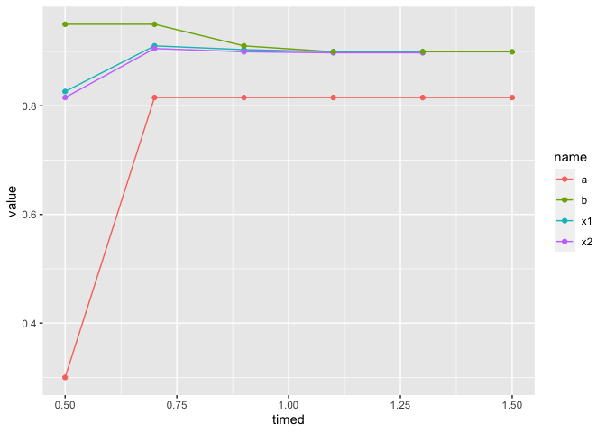
# add lines and points to create plot pre embellishments
# points could be shaped or colored, but overlap, which
# would require them to be jittered away from their lines

p + geom_line() + geom_point()
#> Warning: Removed 2 row(s) containing missing values (geom_path).
#> Warning: Removed 2 rows containing missing values (geom_point).

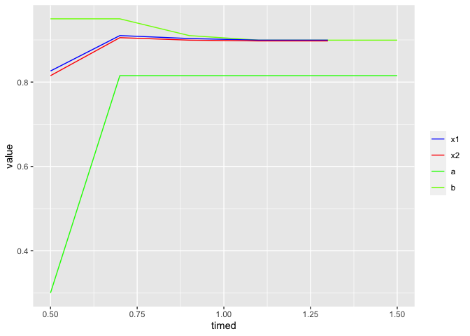
# set line colors and label order
p + geom_line() +
  scale_color_manual(values = c("blue","red","green","lawngreen"),
                     limits = c("x1","x2","a","b"), name = "")
#> Warning: Removed 2 row(s) containing missing values (geom_path).

# position and embellish legend
p + geom_line() +
  scale_color_manual(values = c("blue","red","green","lawngreen"),
                     limits = c("x1","x2","a","b"), name = "") +
  theme(legend.position = c(.97,.123),
      legend.background = element_rect(fill = "white", color = "black"),
)
#> Warning: Removed 2 row(s) containing missing values (geom_path).

# set scales for axes
p + geom_line() +
  scale_x_continuous(breaks = c(0.5,0.6,0.8,1.0,1.2,1.4,1.5)) +
  scale_y_continuous(breaks = c(0.3,0.8,0.82,0.9,0.95))  +
  scale_color_manual(values = c("blue","red","green","lawngreen"),
                     limits = c("x1","x2","a","b"), name = "") +
  theme(legend.position = c(.97,.123),
        legend.background = element_rect(fill = "white", color = "black"),
  )
#> Warning: Removed 2 row(s) containing missing values (geom_path).

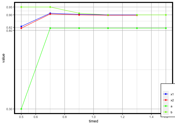
# set panel background to white with gray grid lines with black border

p + geom_line() + geom_point() +
  scale_x_continuous(breaks = c(0.5,0.6,0.8,1.0,1.2,1.4,1.5)) +
  scale_y_continuous(breaks = c(0.3,0.8,0.82,0.9,0.95))  +
  scale_color_manual(values = c("blue","red","green","lawngreen"),
                     limits = c("x1","x2","a","b"), name = "") +
  theme(legend.position = c(.97,.123),
        legend.background = element_rect(fill = "white", color = "black"),
        panel.background = element_rect(fill = "white"),
        panel.grid.major = element_line(color = "gray"),
        panel.grid.minor = element_line(colour = "lightgray"),
        panel.border = element_rect(colour = "black", fill = NA, size = 2.75)
  )
#> Warning: Removed 2 row(s) containing missing values (geom_path).

#> Warning: Removed 2 rows containing missing values (geom_point).

# set labels
x_lab <-  "Time Period (t)"
y_lab <-  "Threshold/Effort Level"
headline <- "Evolution of Legal Threshold and Effort Levels"
subdeck <- "Prepared by ____________, 2020-03-20"
p + geom_line() + geom_point() +
  scale_x_continuous(breaks = c(0.5,0.6,0.8,1.0,1.2,1.4,1.5)) +
  scale_y_continuous(breaks = c(0.3,0.8,0.82,0.9,0.95))  +
  scale_color_manual(values = c("blue","red","green","lawngreen"),
                     limits = c("x1","x2","a","b"), name = "") +
  theme(legend.position = c(.97,.123),
        legend.background = element_rect(fill = "white", color = "black"),
        panel.background = element_rect(fill = "white"),
        panel.grid.major = element_line(color = "gray"),
        panel.grid.minor = element_line(colour = "lightgray"),
        panel.border = element_rect(colour = "black", fill = NA, size = 2.75)
  ) +
  labs(title = headline, subtitle = subdeck) + xlab(x_lab) +  ylab(y_lab)
#> Warning: Removed 2 row(s) containing missing values (geom_path).

#> Warning: Removed 2 rows containing missing values (geom_point).

^{Created on 2020-03-20 by the reprex package (v0.3.0)}

[NathanS]

Sorry for the late response, but thank you so much for these examples!!

[technocrat]

It's going to require some tweaking to get where you're looking. As I mentioned, the viewport differs by device, so I got a better result in the regular R console than I did in RStudio. You'll be able to spot the lines easily to assign the palette and order the variables non-alphabetically.

Taking a look at help(theme) will give you the dizzying array of ways to create a plot available. My regexp was meant as an example of isolating the changeable embellishments to stand alone variables to avoid the finger damage of the plague of quotation marks and parens, and second, to change just one feature at a time.

And I should have emphasized that the colors need to be unique for each variable. Fortunately there are enough closely similar greens in your case.

Use

colors()

It was a good exercise for me. I never tried making all of these adjustment in one go, and I learned a lot.

Thanks.

[technocrat]

No worries. The point underlying is that ggplot is like a language with parts of speech. Learning it is easier if you start with words, then sentences before moving on to paragraphs