multiple regression (testing part)

Please see the below code, I used the "mtcars" dataset to make a multiple regression model, Also I made a vector named Price and assigned some random variables. The Price vector is observation or Y. The mtcars dataset is the feature matrix. I would like to model (B0 + B1.a1 + B2.a2 + ........ + Bn. an = Y).
I splited the data to train and test part, I wrote the train part, How to test the model, Could you please help me?

mtcar = mtcars
number_rows = nrow(mtcar)
print("## number of rows in Train dataset ##")
number_rows_train = 0.7 * number_rows
number_rows_train = ceiling(number_rows_train)
print(number_rows_train)
Train_data = mtcars[1: number_rows_train,]
print("## Head of Train dataset ##")
print(head(Train_data))
print("## number of rows in Test dataset ##")
number_rows_test = number_rows - number_rows_train
print(number_rows_test)
print("## Head of Test dataset ##")
Test_data = mtcars[(number_rows_train+1) : number_rows ,]
print(head(Test_data))

#Whole Response data (I assign some random price to Price vector myself)
Price <- sample(400 : 2500, size = 32)
responce_train = Price[1: number_rows_train]
responce_test = Price [(number_rows_train+1) : number_rows]

model_train = lm(responce_train ~ mpg+cyl+disp+hp+drat+wt+qsec+vs+am+gear+carb,Train_data)
print(model_train)

cat("# # # # The Beta Coefficient Values (Training Part) # # # ","\n")
Beta_coef <- coef(model_train)
print(Beta_coef)
print("----------------------------------------------")
print("Intercept is:")
print(Beta_coef[1]) #the mean value of the response variable when 
                      #all of the predictor variables in the model are equal to zero.
print("----------------------------------------------")
1 Like

I start from your codes;

mtcar = mtcars
number_rows = nrow(mtcar)
print("## number of rows in Train dataset ##")
#> [1] "## number of rows in Train dataset ##"
number_rows_train = 0.7 * number_rows
number_rows_train = ceiling(number_rows_train)
print(number_rows_train)
#> [1] 23
Train_data = mtcars[1: number_rows_train,]
print("## Head of Train dataset ##")
#> [1] "## Head of Train dataset ##"
print(head(Train_data))
#>                    mpg cyl disp  hp drat    wt  qsec vs am gear carb
#> Mazda RX4         21.0   6  160 110 3.90 2.620 16.46  0  1    4    4
#> Mazda RX4 Wag     21.0   6  160 110 3.90 2.875 17.02  0  1    4    4
#> Datsun 710        22.8   4  108  93 3.85 2.320 18.61  1  1    4    1
#> Hornet 4 Drive    21.4   6  258 110 3.08 3.215 19.44  1  0    3    1
#> Hornet Sportabout 18.7   8  360 175 3.15 3.440 17.02  0  0    3    2
#> Valiant           18.1   6  225 105 2.76 3.460 20.22  1  0    3    1
print("## number of rows in Test dataset ##")
#> [1] "## number of rows in Test dataset ##"
number_rows_test = number_rows - number_rows_train
print(number_rows_test)
#> [1] 9
print("## Head of Test dataset ##")
#> [1] "## Head of Test dataset ##"
Test_data = mtcars[(number_rows_train+1) : number_rows ,]
print(head(Test_data))
#>                   mpg cyl  disp  hp drat    wt  qsec vs am gear carb
#> Camaro Z28       13.3   8 350.0 245 3.73 3.840 15.41  0  0    3    4
#> Pontiac Firebird 19.2   8 400.0 175 3.08 3.845 17.05  0  0    3    2
#> Fiat X1-9        27.3   4  79.0  66 4.08 1.935 18.90  1  1    4    1
#> Porsche 914-2    26.0   4 120.3  91 4.43 2.140 16.70  0  1    5    2
#> Lotus Europa     30.4   4  95.1 113 3.77 1.513 16.90  1  1    5    2
#> Ford Pantera L   15.8   8 351.0 264 4.22 3.170 14.50  0  1    5    4

#Whole Response data (I assign some random price to Price vector myself)
Price <- sample(400 : 2500, size = 32)
responce_train = Price[1: number_rows_train]
responce_test = Price [(number_rows_train+1) : number_rows]

model_train = lm(responce_train ~ mpg+cyl+disp+hp+drat+wt+qsec+vs+am+gear+carb,Train_data)
print(model_train)
#> 
#> Call:
#> lm(formula = responce_train ~ mpg + cyl + disp + hp + drat + 
#>     wt + qsec + vs + am + gear + carb, data = Train_data)
#> 
#> Coefficients:
#> (Intercept)          mpg          cyl         disp           hp         drat  
#>   -1857.479       32.837      -22.572       -1.152        5.711     -746.254  
#>          wt         qsec           vs           am         gear         carb  
#>     251.611       50.775     -263.074     -113.935      903.106       46.744

cat("# # # # The Beta Coefficient Values (Training Part) # # # ","\n")
#> # # # # The Beta Coefficient Values (Training Part) # # #
Beta_coef <- coef(model_train)
print(Beta_coef)
#>  (Intercept)          mpg          cyl         disp           hp         drat 
#> -1857.478896    32.836870   -22.572199    -1.151534     5.710904  -746.254309 
#>           wt         qsec           vs           am         gear         carb 
#>   251.611297    50.774756  -263.073837  -113.934830   903.105852    46.744417
print("----------------------------------------------")
#> [1] "----------------------------------------------"
print("Intercept is:")
#> [1] "Intercept is:"
print(Beta_coef[1]) #the mean value of the response variable when 
#> (Intercept) 
#>   -1857.479
#all of the predictor variables in the model are equal to zero.
print("----------------------------------------------")
#> [1] "----------------------------------------------"


#============== Test the model or call it Prediction part ======================
#==================== Use coefficients obtained from Training with =============
#============= their corresponding variables from Testing data sets ============
# Use y = a + Bx {ie, y = a + b1*x1 + b2*x2 + .....}
pred_test = Beta_coef[1] + Test_data['mpg']*Beta_coef[2] + Test_data['cyl']*Beta_coef[3] + 
  Test_data['disp']*Beta_coef[4] + Test_data['hp']*Beta_coef[5] + Test_data['drat']*Beta_coef[6] + 
  Test_data['wt']*Beta_coef[7] + Test_data['qsec']*Beta_coef[8] + Test_data['vs']*Beta_coef[9] + 
  Test_data['am']*Beta_coef[10] + Test_data['gear']*Beta_coef[11] + Test_data['carb']*Beta_coef[12]

# Compare the reserved data for testing with the new predictions
df_com_test <- data.frame(pred_test, 'obs' = responce_test) # pred_test is your new predictions
names(df_com_test)[names(df_com_test) == 'mpg'] <- 'pred' # Convert rownames to column ids
df_com_test['ID']  <- rownames(df_com_test)
# Now go on plotting/analysing your 'df_com_test' with your statistical measures like correlation, RMSE etc

df_melt <- reshape2::melt(df_com_test, id = 'ID')
ggplot2::ggplot(data = df_melt, aes(x = ID, y = value, group = variable, color = variable)) +
  geom_line( size = 1) + geom_point(size = 2)
#> Error in aes(x = ID, y = value, group = variable, color = variable): could not find function "aes"

Please note that for an elegant regression analysis using multiple predictors, I suggest you to look for another response of mine at nls fit function with summation

If you have any more doubt please drop your concern(s) down .....

1 Like

Thank you so much, I ran it and saw the plot. It was really nice.
Actually, I didn't work on the regression model, but a couple of years ago I worked on classification models, so I forgot the machine learning concepts. As far as I remember for classification we calculate the accuracy of the model, for example, 92%. I mean we reached a specific number. is it correct in Regression as well? how can I find it in this problem?

second question: could you please write the testing part generally, because I want to use it for another large dataset in which the number of predictors is more than 100.
this section:

pred_test = Beta_coef[1] + Test_data['mpg']*Beta_coef[2] + Test_data['cyl']*Beta_coef[3] + 
  Test_data['disp']*Beta_coef[4] + Test_data['hp']*Beta_coef[5] + Test_data['drat']*Beta_coef[6] + 
  Test_data['wt']*Beta_coef[7] + Test_data['qsec']*Beta_coef[8] + Test_data['vs']*Beta_coef[9] + 
  Test_data['am']*Beta_coef[10] + Test_data['gear']*Beta_coef[11] + Test_data['carb']*Beta_coef[12]

Thank you in advance.

1 Like

You can use the predict() function to calculate predicted values from a model. For example, to get the y values (Price) predicted by the model using your Test_data you can use.

PredictedTest <- predict(model_train, newdata = Test_data)

One way to characterize the quality of the prediction is to calculate the Mean Squared Error MSE. You have the responce_test values and the PredictedTest values. You can subtract those two, square the result and get the MSE from that.

3 Likes

As @FJCC commented, you can use MSE/RMSE to evaluate the performance of your model. In your case, it seems that you are looking for a significant test at some levels, say 95%. In that case, you can use "confint" function to achieve that.

To answer your queries, try to follow the codes below;

df <- mtcars
df['price'] <- sample(400 : 2500, size = nrow(df)) # Add a column of price just as you did.

# Splitting data for train and test
ind <- sample(nrow(df), size = 0.7*nrow(df), replace = F) # We use 70% of the df in Training
df_Train <- df[ind, ]
df_Test <- df[-ind, ]

# Train/Develop the model. We use all predictors in df, with price as predictand/response

fit_model <- lm(price ~., data = df_Train)   # Build the model
# Note that, not all variables can influence your response. 
summary(fit_model) # See the summary. 
#> 
#> Call:
#> lm(formula = price ~ ., data = df_Train)
#> 
#> Residuals:
#>    Min     1Q Median     3Q    Max 
#> -893.6 -310.7 -106.2  463.0  929.8 
#> 
#> Coefficients: (1 not defined because of singularities)
#>               Estimate Std. Error t value Pr(>|t|)
#> (Intercept) 20369.9266 18509.6209   1.101    0.295
#> mpg            43.1637    80.5942   0.536    0.603
#> cyl           -13.6964   466.4630  -0.029    0.977
#> disp            0.4528     5.4551   0.083    0.935
#> hp            -22.1046    15.1269  -1.461    0.172
#> drat         -784.2134   767.5272  -1.022    0.329
#> wt           1032.8341   927.6895   1.113    0.289
#> qsec         -983.6680   783.9803  -1.255    0.236
#> vs           2195.7889  1226.8170   1.790    0.101
#> am                  NA         NA      NA       NA
#> gear         -401.9742  1042.7835  -0.385    0.707
#> carb          179.6202   378.8715   0.474    0.645
#> 
#> Residual standard error: 694.4 on 11 degrees of freedom
#> Multiple R-squared:  0.3338, Adjusted R-squared:  -0.2719 
#> F-statistic: 0.5511 on 10 and 11 DF,  p-value: 0.8214
# You need predictors with at least one (1) star after column Pr(>|t|) from summary.
# In this case it seems all our predictors are insignificant, since no any star at the end from summary.
# Alternatively you can use the package "relaimpo" to calculate/identify the importances of your predictors

# Also you can see other informations from your fit model. 
fit_model$coefficients
#>   (Intercept)           mpg           cyl          disp            hp 
#> 20369.9266334    43.1636595   -13.6964068     0.4527914   -22.1045852 
#>          drat            wt          qsec            vs            am 
#>  -784.2134301  1032.8341046  -983.6680210  2195.7889354            NA 
#>          gear          carb 
#>  -401.9741836   179.6202151
fit_model$effects ; # etc Use fit_model$xxxxx to see other information
#> (Intercept)         mpg         cyl        disp          hp        drat 
#> -5994.77774    10.74388   407.84285   -50.38455   402.13553   280.52474 
#>          wt        qsec          vs        gear        carb             
#>  -570.41721  -168.51445 -1335.25978    56.75030  -329.23028  -699.83919 
#>                                                                         
#>   475.19803   556.15428   201.00593  -210.30365   759.28810  1303.91192 
#>                                                 
#>  -763.31647   110.00162   545.77770  1012.86774

# Also you can check the the confidence interval from your model 
confint(fit_model) 
#>                    2.5 %      97.5 %
#> (Intercept) -20369.47434 61109.32760
#> mpg           -134.22302   220.55034
#> cyl          -1040.37465  1012.98183
#> disp           -11.55385    12.45943
#> hp             -55.39875    11.18958
#> drat         -2473.52946   905.10259
#> wt           -1008.99661  3074.66482
#> qsec         -2709.19708   741.86104
#> vs            -504.41701  4895.99488
#> am                    NA          NA
#> gear         -2697.12529  1893.17692
#> carb          -654.27023  1013.51066
confint(fit_model, level = .95)  
#>                    2.5 %      97.5 %
#> (Intercept) -20369.47434 61109.32760
#> mpg           -134.22302   220.55034
#> cyl          -1040.37465  1012.98183
#> disp           -11.55385    12.45943
#> hp             -55.39875    11.18958
#> drat         -2473.52946   905.10259
#> wt           -1008.99661  3074.66482
#> qsec         -2709.19708   741.86104
#> vs            -504.41701  4895.99488
#> am                    NA          NA
#> gear         -2697.12529  1893.17692
#> carb          -654.27023  1013.51066
# Type help(confint) of ??confint for help

# Test the model/Predicting
# You can use predict() from base-R package called "stats" which loads by deafult
pred_model <- predict(fit_model, newdata = df_Test)  # 
#> Warning in predict.lm(fit_model, newdata = df_Test): prediction from a rank-
#> deficient fit may be misleading

# Get the data for further analysis
df_anly <- data.frame(df_Test['price'], 'pred' = pred_model)
df_anly['Names'] <- rownames(df_anly) 

reshape2::melt(df_anly, id = 'Names') |> 
  ggplot2::ggplot( aes( x = Names, y = value, group = variable, color = variable) ) +
  geom_line(size = 1) + geom_point(size = 2)

# Let us assess the performance of our developed model using RMSE
rmse1 <- sqrt(mean((df_anly$pred - df_anly$price)**2))
print(rmse1)
#> [1] 1751.047

# Here I use the 'measures' package to calculate the RMSE 
rmse2 <- measures::RMSE(truth = df_anly$price, response = df_anly$pred) 
print(rmse2)
#> [1] 1751.047

Alternatively, you can use matrix multiplications for multiple predictors. Just see my response at nls fit function with summation - #2 by pe2ju. Here I post the workaround;

Suppose your data is in Matrix form and use Matrix Multiplications to perform the linear regressions. Suppose a data frame of 2 predictors/regressors and the parameters 'a' as a constant and coefficients B [b1 and b2] since we have 2 regressors. Then, you go smoothly as follows;

predic <- data.frame( 'Model_01' = rnorm(50, mean = 4.5, sd = 1.5 ),
                      'Model_02' = rnorm(50, mean = 3.5, sd = 1.2 ) )
predic2Mat <- as.matrix(predic, byrow = F)
predic2Mat <- cbind(rep(1, nrow(predic2Mat)), predic2Mat) # We add 1 for mutrix multiplications

pars <- c('a' = 2, 'b1' = 3.5, 'b2' = 1.8) # a = constant, b1 & b2 are coefficients from your model 

new_pred <- predic2Mat %*% pars  # Get the new predictions

For further useful elaborations on Linear Regression. Just follow these links;

https://rpubs.com/aaronsc32/regression-confidence-prediction-intervals#:~:text=To%20find%20the%20confidence%20interval,to%20output%20the%20mean%20interval
1 Like

Thank you so much for your help :slight_smile:

1 Like

@pe2ju
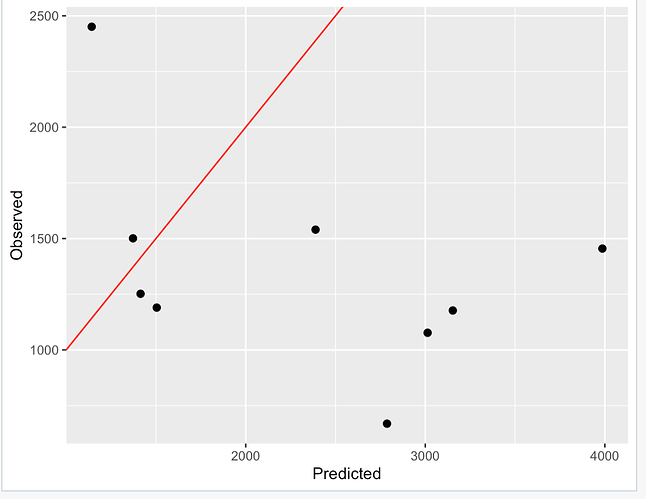
Is there a way to show the plot in another way, I mean is it possible to show predicted values on the X-axis and observed values on the Y-axis?

1 Like

You can interchange x for y as follows, Or you can any kind of plotting approach(es) of your preferences like base-R plottings.

@pe2ju
Please see the figure, every time that I run the code, the plot is different, is it right or have I made a mistake?


the reason is the different Beta coefficient?

If you are using the codes above, then it is possible to have different results whenever you run the code. This is because the generation of your response variable as well as the splitting process uses random seeds. So, in order to have the same results for reproducibility, you need to fix the number of seeds. Check the modified code here and run it as many times as you wish, you will end up with the same results.

The rest goes as is.

This topic was automatically closed 7 days after the last reply. New replies are no longer allowed.

If you have a query related to it or one of the replies, start a new topic and refer back with a link.