Markdown datatable and plots not rendered correctly

Hi folks,
I was trying to produce a .Rmd template to use for generating an html report of my RNAseq analyses.
This output should include a data frame with the results (rendered with the command DT::datatable) followed by a set of plots related to that data frame.

An example of my .Rmd code is:


title: ""
author: "r paste0('GeneTonic happy_hour (v', utils::packageVersion('GeneTonic'), ')')"
date: "r Sys.Date()"

output:
html_document:
toc: true
toc_float: true
code_folding: hide
code_download: false
number_sections: true
df_print: kable
theme: lumen
always_allow_html: yes

knitr::opts_chunk$set(
  echo = TRUE, 
  warning = FALSE, 
  message = FALSE,
  error = TRUE
)
# knitr::opts_knit$set(
#   progress = FALSE, 
#   verbose = FALSE
# )
rm(list=ls())
library(GeneTonic)
library("macrophage")
library("DESeq2")
library("org.Hs.eg.db")
library("AnnotationDbi")

Preparing the required data:

# dds object
data("gse", package = "macrophage")
dds_macrophage <- DESeqDataSet(gse, design = ~ line + condition)
rownames(dds_macrophage) <- substr(rownames(dds_macrophage), 1, 15)
dds_macrophage <- estimateSizeFactors(dds_macrophage)

vst_data <- vst(dds_macrophage)

# annotation object
anno_df <- data.frame(
  gene_id = rownames(dds_macrophage),
  gene_name = mapIds(org.Hs.eg.db,
                     keys = rownames(dds_macrophage),
                     column = "SYMBOL",
                     keytype = "ENSEMBL"
  ),
  stringsAsFactors = FALSE,
  row.names = rownames(dds_macrophage)
)


# res object
data(res_de_macrophage, package = "GeneTonic")
res_de <- res_macrophage_IFNg_vs_naive

# res_enrich object
data(res_enrich_macrophage, package = "GeneTonic")
res_enrich <- shake_topGOtableResult(topgoDE_macrophage_IFNg_vs_naive)
res_enrich <- get_aggrscores(res_enrich, res_de, anno_df)

# gtl list:
gtl <- GeneTonicList(
  dds = dds_macrophage,
  res_de = res_de,
  res_enrich = res_enrich,
  annotation_obj = anno_df
)

Plotting the data:

cat("  \nDataframe of the results is here:")
print(htmltools::tagList(DT::datatable(res_enrich)))

#### ~~~ MDS: ~~~ ####
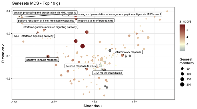
cat("  \n**Geneset MDS plot**: A Multi Dimensional Scaling plot for gene sets. Color coded by the *[z-score](http://www.bioconductor.org/packages/release/bioc/vignettes/GeneTonic/inst/doc/GeneTonic_manual.html#2_Getting_started)* (a score attempts to determine the “direction” of change")
print(gs_mds(gtl = gtl,
             mds_colorby = 'z_score',
             mds_labels = 10,
             plot_title = "Genesets MDS - Top 10 gs"))


#### ~~~ENRICHMENT MAP: ~~~ ####
cat("  \n**Enrichment map**: An interactive plot which shows the relationship between genesets (more info [here](https://journals.plos.org/plosone/article?id=10.1371/journal.pone.0013984)). Genesets are dots and the segment that connect genesets indicate shared genes between genesets.  
      Only the first 50 gene sets are included in the plot, and are color-coded by their p-value.  \n")
em <- enrichment_map(gtl = gtl,
                     n_gs = 50,
                     overlap_threshold = 0.1,
                     scale_edges_width = 200,
                     color_by = 'gs_pvalue',
                     scale_nodes_size = 5,
)
library("igraph")
library("visNetwork")
library("magrittr")

print(htmltools::tagList(em %>% # To print this, see this post https://stackoverflow.com/questions/60685631/using-ggplotly-and-dt-from-a-for-loop-in-rmarkdown
                           visIgraph() %>% 
                           visOptions(highlightNearest = list(enabled = TRUE,
                                                              degree = 1,
                                                              hover = TRUE),
                                      nodesIdSelection = TRUE) %>%
                           visExport(
                             name = 'emap_network',
                             type = 'pdf',
                             label = 'Save enrichment map'
                           )))

#### ~~~ ENHANCED TABLE: ~~~ ####
cat("  \n**Enhanced table** summarising the genesets displaying the `logFC` of each set's component. Each gene is a dot on the plot. Only the first 15 genesets are shown. N.B. It is an interactive plot.  \n")
print(htmltools::tagList(plotly::ggplotly(enhance_table(gtl=gtl,
                                                        n_gs = 15,
                                                        chars_limit = 50,
                                                        plot_title = "Enrichment overview = Top 15 gs")) ))

#### ~~~ DENDROGRAM: ~~~ ####
cat("  \n**Geneset dendrogram**: this plot creates a tree with significant genesets. Works only with the Gene Onthology database. Only the first 25 gene sets are included in the plot.  \n")
gs_dendro(gtl = gtl, n_gs = 25) 


#### ~~~ SCORES HEATMAP: ~~~ ####
cat("  \n**Scores Heatmap**: this plot uses the `z-score` and shows on an heatmap the degree of activation/deactivation of pathways in each sample. Only the first 15 gene sets are included in the plot.  \n")
gss_mat <- gs_scores(
  se = vst_data,
  gtl = gtl)

scoresheat = gs_scoresheat(
  #gss_mat[, order(colnames(gss_mat))], #to alphabetically order colnames.
  #cluster_cols = F, #Leave F if you want to alphabetically order colnames
  gss_mat,
  n_gs = 15,
  cluster_cols = T,
) + ggplot2::theme_bw() + 
  ggpubr::rotate_x_text(45) +
  ggplot2::ggtitle("Scores Heatmap - Top 15 gs")
print(scoresheat)

Basically if I run the last chunk by pressing the "Run Current Chunk" button, the datatable and plots are all correctly produced. However if I knit the document the table is not displayed and only the MDS, dendrogram and scores heatmap plots are displayed...

I have Rstudio 2023.03.0+386, R 4.2.1 and I am running a MacOS 12.6.5.
Can somebody help me?
Any help will be much appreciated
Thanks
Luca
I've installed the required packages and put your code in a new rmd document. Because it outputs raw html in part I can't tell exactly where the problem arises.

My suggestion is to go back and discard the cat and print statements that do anything in the way of attempting to display objects, such as

print(htmltools::tagList(DT::datatable(res_enrich)))

To display a DT table in rmd all that's needed is

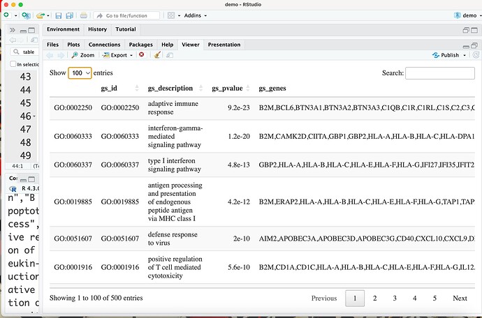
DT::datatable(res_enrich)

Will display output that looks like the following image

Thanks @technocrat! Your suggestion to get rid of all the print and print(htmltools::tagList statements works. If I get rid of them the plots are all correctly shown in the html report. I have kept the cat statements as they worked fine.

However I have another problem. I have several (i.e. from 2 to 6 depending on the input data) possible res_enrich data frames and I would like to produce the datatable and figures for each of them, without the need to edit my Rmd every time.

My res_enrich df are stored in a list (as you can see from my code).


MY .RMD CODE:


title: ""
author: "r paste0('GeneTonic happy_hour (v', utils::packageVersion('GeneTonic'), ')')"
date: "r Sys.Date()"

output:
html_document:
toc: true
toc_float: true
code_folding: hide
code_download: false
number_sections: true
df_print: kable
theme: lumen
always_allow_html: yes

knitr::opts_chunk$set(
  echo = TRUE, 
  warning = FALSE, 
  message = FALSE,
  error = TRUE
)
# knitr::opts_knit$set(
#   progress = FALSE, 
#   verbose = FALSE
# )
rm(list=ls())
library(GeneTonic)
library("macrophage")
library("DESeq2")
library("org.Hs.eg.db")
library("AnnotationDbi")
library(DT)

Custom function:

ProcessResults <- function(res_enrich_name, functional_data = list_FA$res_ORA, Functional_analysis, outdf=T, outplot=T){
  
  # 0. check df is not empty
  cat(paste0("\n\n### ", res_enrich_name, "\n"))
  df = as.data.frame(functional_data[[res_enrich_name]])
  if (nrow(df) == 0){
    outdf = F; outplot = F
    cat("No enriched pathways for this gene list...")
  }
  
  # 1. print table:
  if(outdf){
    datatable(df)
  }
  
  # 2. shake_results:
  if(outplot){
    
    
    # 3. Make gtl:
    gtl = GeneTonic_list(dds = dds_macrophage, 
                         res_de = res_de,
                         res_enrich = res_enrich,
                         annotation_obj = anno_df)
    
    #MDS:
    
    cat(("\n\n#### Geneset MDS plot\n"))
    
    cat(paste0("**Geneset MDS plot**: A Multi Dimensional Scaling plot for gene sets. Color coded by the *[z-score](http://www.bioconductor.org/packages/release/bioc/vignettes/GeneTonic/inst/doc/GeneTonic_manual.html#2_Getting_started)* (a score attempts to determine the “direction” of change: positive score means that genes are mostly up-regulated in the first term.  \n"))
    
    gs_mds(gtl = gtl,
                 mds_colorby = 'z_score',
                 mds_labels = 10,
                 plot_title = "Genesets MDS - Top 10 gs")
    
    
    #ENRICHMENT MAP:
    
    cat(("\n\n#### Enrichment map\n"))
    
    cat("**Enrichment map**: An interactive plot which shows the relationship between genesets (more info [here](https://journals.plos.org/plosone/article?id=10.1371/journal.pone.0013984)). Genesets are dots and the segment that connect genesets indicate shared genes between genesets.  
      Only the first 50 gene sets are included in the plot, and are color-coded by their p-value.  \n")
    em <- enrichment_map(gtl = gtl,
                         n_gs = 50,
                         overlap_threshold = 0.1,
                         scale_edges_width = 200,
                         color_by = 'gs_pvalue',
                         scale_nodes_size = 5)
    library("igraph")
    library("visNetwork")
    library("magrittr")
    
    em %>% 
      visIgraph() %>% 
      visOptions(highlightNearest = list(enabled = TRUE,
                                         degree = 1,
                                         hover = TRUE),
                 nodesIdSelection = TRUE) %>%
      visExport(
        name = 'emap_network',
        type = 'pdf',
        label = 'Save enrichment map')
    
    #ENHANCED TABLE:
    
    cat(("\n\n#### Enhanced table\n"))
    
    cat("  \n**Enhanced table** summarising the genesets displaying the `logFC` of each set's component. Each gene is a dot on the plot. Only the first 15 genesets are shown. N.B. It is an interactive plot.  \n")
    plotly::ggplotly(enhance_table(gtl=gtl,
                                                            n_gs = 15,
                                                            chars_limit = 50,
                                                            plot_title = "Enrichment overview = Top 15 gs"))
    
    #DENDROGRAM:
    cat(("\n\n#### Dendrogram\n"))
    
    cat("  \n**Geneset dendrogram**: this plot creates a tree with significant genesets. Works only with the Gene Onthology database. Only the first 25 gene sets are included in the plot.  \n")
    gs_dendro(gtl = gtl, n_gs = 25) 
    
  
    #SCORES HEATMAP:
    cat(("\n\n### Scores Heatmap\n"))
    
    cat("**Scores Heatmap**: this plot uses the `z-score` and shows on an heatmap the degree of activation/deactivation of pathways in each sample. Only the first 15 gene sets are included in the plot.  \n")
    gss_mat <- gs_scores(
      se = vst_data,
      gtl = gtl)
    
    gs_scoresheat(
      #gss_mat[, order(colnames(gss_mat))], #to alphabetically order colnames.
      #cluster_cols = F, #Leave F if you want to alphabetically order colnames
      gss_mat,
      n_gs = 15,
      cluster_cols = T) + 
      ggplot2::theme_bw() + 
      ggpubr::rotate_x_text(45) +
      ggplot2::ggtitle("Scores Heatmap - Top 15 gs")
  }
}

Preparing the required data:

# dds object
data("gse", package = "macrophage")
dds_macrophage <- DESeqDataSet(gse, design = ~ line + condition)
rownames(dds_macrophage) <- substr(rownames(dds_macrophage), 1, 15)
dds_macrophage <- estimateSizeFactors(dds_macrophage)

vst_data <- vst(dds_macrophage)

# annotation object
anno_df <- data.frame(
  gene_id = rownames(dds_macrophage),
  gene_name = mapIds(org.Hs.eg.db,
                     keys = rownames(dds_macrophage),
                     column = "SYMBOL",
                     keytype = "ENSEMBL"
  ),
  stringsAsFactors = FALSE,
  row.names = rownames(dds_macrophage)
)


# res object
data(res_de_macrophage, package = "GeneTonic")
res_de <- res_macrophage_IFNg_vs_naive

# res_enrich object
data(res_enrich_macrophage, package = "GeneTonic")
res_enrich <- shake_topGOtableResult(topgoDE_macrophage_IFNg_vs_naive)
res_enrich <- get_aggrscores(res_enrich, res_de, anno_df)

Example of several res_enrich objects:

# example list of res_enrich objects:
res_enrich.list = list()
res_enrich.1 = res_enrich[1:145,]
res_enrich.2 = res_enrich[146:300,]
res_enrich.3 = res_enrich[301:500,]

res_enrich.list = append(res_enrich.list, list(res1 = res_enrich.1))
res_enrich.list = append(res_enrich.list, list(res1 = res_enrich.2))
res_enrich.list = append(res_enrich.list, list(res1 = res_enrich.3))

Looping through the res_enrich objects:

for (name in names(res_enrich.list)){
  ProcessResults(res_enrich_name = name, functional_data = res_enrich.list, Functional_analysis="ora")
}

Or, without the for loop. Just by using the function:

ProcessResults(res_enrich_name = "res1", functional_data = res_enrich.list, Functional_analysis="ora")

END OF .RMD


Because I have several res_enrich db I have written a function to include all the relevant steps (outputting datatable and plots) and loop through the different res_enrich objects generating the desired results via the code:

for (name in names(res_enrich.list)){ 
  ProcessResults(res_enrich_name = name, functional_data = res_enrich.list, Functional_analysis="ora")
}

However this does not produce the plots (more specifically the Enrichment map and Enhanced table, which are the interactive plots) when I knit the document.
I have also tried using the function outside the for ... loop in this way:

ProcessResults(res_enrich_name = "res1", functional_data = res_enrich.list, Functional_analysis="ora")

But also in this case when I knit I do not get the desired output plots (which are the same as the case above). Further, even if I press the "Run current chunk" button on a chunk that contains only this line of code (r ProcessResults(res_enrich_name = "res1", functional_data = res_enrich.list, Functional_analysis="ora") ) the same situation happens (no interactive plots being plotted). I suspect this has to do with the fact that I am including the plots inside a function.

Does anyone have some suggestions on how to solve this problem by keeping in mind that I have a variable number of res_enrich data frames and I would prefer to avoid having to copy/paste the previous code for each of my res_enrich objects.

Thanks a lot
Luca

How do the results escape the loop into the .Global environment?

Ehm, honestly I don't know.

But it doesn't work also if I take the function and execute it outside the for loop (only by executing it on one res_enrich object. That is why I had originally added the print statements (the ones on my first post here)

If this works when you substitute name = res_enrich.list[SOMETHING] then the for` loop will return at most one name . Try creating a receptor list

r <- vector(length = [number of names in your object

then

for (name in names(res_enrich.list)){
  r[name] = ProcessResults(res_enrich_name = name, functional_data = res_enrich.list, Functional_analysis="ora")
}

Dear @technocrat,
Thanks for your reply. I have put, as you suggested, the elements into a receptor list by editing the ProcessResults.list function. Now it returns a list of objects (one data frame and the plots that I would like to render in the final html output).

I can loop through all the res_enrich objects so that a list for each res_enrich is created and nested within a list_outputs_ORA object (see below).

Now my question is: how can I effectively render the plots and tables?
Thanks again for your patience and help

Luca


title: ""
author: "r paste0('GeneTonic happy_hour (v', utils::packageVersion('GeneTonic'), ')')"
date: "r Sys.Date()"

output:
html_document:
toc: true
toc_float: true
code_folding: hide
code_download: false
number_sections: true
df_print: kable
theme: lumen
always_allow_html: yes

knitr::opts_chunk$set(
  echo = TRUE, 
  warning = FALSE, 
  message = FALSE,
  error = TRUE
)
# knitr::opts_knit$set(
#   progress = FALSE, 
#   verbose = FALSE
# )
rm(list=ls())
library(GeneTonic)
library("macrophage")
library("DESeq2")
library("org.Hs.eg.db")
library("AnnotationDbi")
library(DT)

Preparing the required data:

# dds object
data("gse", package = "macrophage")
dds_macrophage <- DESeqDataSet(gse, design = ~ line + condition)
rownames(dds_macrophage) <- substr(rownames(dds_macrophage), 1, 15)
dds_macrophage <- estimateSizeFactors(dds_macrophage)

vst_data <- vst(dds_macrophage)

# annotation object
anno_df <- data.frame(
  gene_id = rownames(dds_macrophage),
  gene_name = mapIds(org.Hs.eg.db,
                     keys = rownames(dds_macrophage),
                     column = "SYMBOL",
                     keytype = "ENSEMBL"
  ),
  stringsAsFactors = FALSE,
  row.names = rownames(dds_macrophage)
)


# res object
data(res_de_macrophage, package = "GeneTonic")
res_de <- res_macrophage_IFNg_vs_naive

# res_enrich object
data(res_enrich_macrophage, package = "GeneTonic")
res_enrich <- shake_topGOtableResult(topgoDE_macrophage_IFNg_vs_naive)
res_enrich <- get_aggrscores(res_enrich, res_de, anno_df)

Example of several res_enrich objects:

# example list of res_enrich objects:
res_enrich.list = list()
res_enrich.1 = res_enrich[1:145,]
res_enrich.2 = res_enrich[146:300,]
res_enrich.3 = res_enrich[301:500,]

res_enrich.list = append(res_enrich.list, list(res1 = res_enrich.1))
res_enrich.list = append(res_enrich.list, list(res2 = res_enrich.2))
res_enrich.list = append(res_enrich.list, list(res3 = res_enrich.3))

Custom function to generate List objects:

ProcessResults.list <- function(res_enrich_name, functional_data = list_FA$res_ORA, Functional_analysis, outdf=T, outplot=T){
  
  resultList=list()
  
  # 0. check df is not empty
  cat(paste0("\n\n### ", res_enrich_name, "\n"))
  df = as.data.frame(functional_data[[res_enrich_name]])
  if (nrow(df) == 0){
    outdf = T; outplot = F
    messaggio = "No significant pathways for this gene list..."
    df = data.frame(messaggio)
  }
  
  # 1. print table:
  if(outdf){
    resultList = append(resultList, list(res_enrich_name = df))
  }
  
  if(outplot){
    
    # 2. Make gtl:
    gtl = GeneTonic_list(dds = dds_macrophage, 
                         res_de = res_macrophage_IFNg_vs_naive,
                         res_enrich = df,
                         annotation_obj = anno_df)
    
    #MDS:
    mds = gs_mds(gtl = gtl,
                 mds_colorby = 'z_score',
                 mds_labels = 10,
                 plot_title = "Genesets MDS - Top 10 gs")
    
    resultList = append(resultList, list(mdsplot = mds))
    
    #ENRICHMENT MAP:
    em <- enrichment_map(gtl = gtl,
                         n_gs = 50,
                         overlap_threshold = 0.1,
                         scale_edges_width = 200,
                         color_by = 'gs_pvalue',
                         scale_nodes_size = 5)
    
    resultList = append(resultList, list(emplot = em))
    
    #ENHANCED TABLE:
    enhantable = enhance_table(gtl=gtl,
                                                            n_gs = 15,
                                                            chars_limit = 50,
                                                            plot_title = "Enrichment overview = Top 15 gs")
    resultList = append(resultList, list(enhanplot = enhantable))
    
    
    #DENDROGRAM:
    dendro = gs_dendro(gtl = gtl, n_gs = 25, create_plot = F) 
    
    resultList = append(resultList, list(dendroplot = dendro))
  
    #SCORES HEATMAP:
    gss_mat <- gs_scores(
      se = vst_data,
      gtl = gtl)
    
    resultList = append(resultList, list(scoresplot = gss_mat))
    
    return(resultList)
  }
}

loop through the res_enrich objects:

list_df = names(res_enrich.list)
list_outputs_ORA= list()
for (i in list_df){
  results = ProcessResults.list(res_enrich_name = i, functional_data = res_enrich.list, Functional_analysis="ora", outplot=T)
  list_outputs_ORA = append(list_outputs_ORA, list(results = results))
  names(list_outputs_ORA)[names(list_outputs_ORA) == "results"] <- i
}

That get's us over one big hump. list_outputs_ORA has the results of the for loop. Next up

That depends on what's in list_outputs_ORA, how to find it and how you want to render it.

For example, there's this plot

and what I imagine to be the related data frame and there are possibly others.

So what parts of list_outputs_ORA are to be rendered will dictate the best way to go about unpacking it. The object is a deeply nested list of lists of lists. I have zero domain knowledge (genes, encoded in segments of my DNA, I'm pretty sure, is about the extent of it) so I have no insight into what parts of the object are of interest.

# trimmed to fit
               gs_id
GO:0002250 GO:0002250
GO:0060333 GO:0060333
GO:0060337 GO:0060337
GO:0019885 GO:0019885
GO:0051607 GO:0051607
GO:0001916 GO:0001916
                                                                             gs_description
GO:0002250                                                          adaptive immune response
GO:0060333                                       interferon-gamma-mediated signaling pathway
GO:0060337                                               type I interferon signaling pathway
GO:0019885 antigen processing and presentation of endogenous peptide antigen via MHC class I
GO:0051607                                                         defense response to virus
GO:0001916                               positive regulation of T cell mediated cytotoxicity
          gs_pvalue
GO:0002250   9.2e-23
GO:0060333   1.2e-20
GO:0060337   4.8e-13
GO:0019885   4.2e-12
GO:0051607   2.0e-10
GO:0001916   5.6e-10
                                                                                                                                                                                                                                                                                                                                                                                                                                                                                                                                                                                 gs_genes
GO:0002250 B2M,BCL6,BTN3A1,BTN3A2,BTN3A3,C1QB,C1R,C1RL,C1S,C2,C3,C4A,C4B,CD1A,CD1C,CD274,CD28,CD40,CD7,CD74,CD80,CEACAM1,CLEC10A,CLEC6A,CTLA4,CTSS,ERAP2,EXO1,FGL1,FGL2,GCNT3,GPR183,HLA-A,HLA-B,HLA-C,HLA-DMA,HLA-DMB,HLA-DOA,HLA-DOB,HLA-DPA1,HLA-DPB1,HLA-DQA1,HLA-DQB1,HLA-DQB2,HLA-DRA,HLA-DRB1,HLA-DRB5,HLA-E,HLA-F,HLA-G,ICAM1,IL12A,IL12RB1,IL18BP,IL27,IRF1,IRF7,ITK,JAK2,JAK3,KLRK1,LAG3,LAMP3,LILRA1,LILRB3,LYN,MCOLN2,P2RX7,PDCD1,PDCD1LG2,RELB,RIPK2,RNF19B,RSAD2,SERPING1,SIT1,SLAMF1,SLAMF6,SLAMF7,SLC11A1,TAP1,TAP2,TBX21,TLR8,TNFRSF11A,TNFRSF21,TNFSF13B,TNFSF18,ZC3H12A
GO:0060333                                                                                                                                                                                                                                                                                                                                                       B2M,CAMK2D,CIITA,GBP1,GBP2,HLA-A,HLA-B,HLA-C,HLA-DPA1,HLA-DPB1,HLA-DQA1,HLA-DQB1,HLA-DQB2,HLA-DRA,HLA-DRB1,HLA-DRB5,HLA-E,HLA-F,HLA-G,ICAM1,IRF1,IRF7,JAK2,MT2A,NLRC5,NMI,OAS2,PARP14,PML,SOCS1,STAT1,TRIM22,TRIM31,VCAM1
GO:0060337                                                                                                                                                                                                                                                                                                                                                                                                                              GBP2,HLA-A,HLA-B,HLA-C,HLA-E,HLA-F,HLA-G,IFI27,IFI35,IFIT2,IFIT3,IFITM1,IFITM2,IFITM3,IRF1,IRF7,ISG20,NLRC5,OAS2,PSMB8,RSAD2,STAT1,STAT2,XAF1,ZBP1
GO:0019885                                                                                                                                                                                                                                                                                                                                                                                                                                                                                                                   B2M,ERAP2,HLA-A,HLA-B,HLA-C,HLA-E,HLA-F,HLA-G,TAP1,TAP2,TAPBP
GO:0051607                                                                                                                                                                                                                                                                                                                  AIM2,APOBEC3A,APOBEC3D,APOBEC3G,CD40,CXCL10,CXCL9,DDX60,DTX3L,FGL2,GBP1,GBP3,IFI27,IFI44L,IFIH1,IFIT2,IFIT3,IFIT5,IFITM1,IFITM2,IFITM3,IL12RB1,IL15,IL27,IRF1,IRF7,ISG20,NLRC5,OAS2,PMAIP1,PML,RSAD2,RTP4,SERINC5,STAT1,STAT2,TLR7,TLR8,TRIM22,TSPAN32,ZC3H12A
GO:0001916                                                                                                                                                                                                                                                                                                                                                                                                                                                                                                           B2M,CD1A,CD1C,HLA-A,HLA-B,HLA-C,HLA-E,HLA-F,HLA-G,IL12A,IL12RB1,P2RX7
          gs_de_count gs_bg_count Expected
GO:0002250          89         323    17.93
GO:0060333          34          82     4.55
GO:0060337          25          80     4.44
GO:0019885          11          14     0.78
GO:0051607          41         206    11.44
GO:0001916          12          23     1.28
          DE_count  z_score aggr_score
GO:0002250       89 7.101986   2.989686
GO:0060333       34 5.830952   4.068646
GO:0060337       25 5.000000   3.338149
GO:0019885       11 3.316625   3.114728
GO:0051607       41 6.090777   3.645270
GO:0001916       12 2.309401   2.250208

I think I figured it out.
The solution was provided here: r - Using `ggplotly` and `DT` from a `for` loop in Rmarkdown - Stack Overflow

I switched to using the print(htmltools::tagList()) statements from my first message. But the trick was to add a chuck to initialise the htmltools at the beginning of the .Rmd like this:

# Init Step to make sure that the dependencies are loaded
htmltools::tagList(datatable(cars))
htmltools::tagList(ggplotly(ggplot()))

This chunk HAS to be outside the for loop. In this way all the plots generated inside the for loop are correctly rendered when I knit the document.

Thanks for your support @technocrat, much appreciated! :grin:

1 Like

This topic was automatically closed 45 days after the last reply. New replies are no longer allowed.

If you have a query related to it or one of the replies, start a new topic and refer back with a link.