Maps with no restrictions and basic code required

Hi,
We are trying to map scores in specific towns and cities. We already excluded ideas of using Google Maps as they have new restrictions in terms of linking maps with any external resources (API registration limits R capabilities).
Can you suggest the best way of displaying scores on any map (maybe using open source such as https://www.openstreetmap.org/). Which package is the easiest to use? Is any package available with an option of simply listing cities or towns (or other regions) without giving specific geographical coordinates?

Would you also be able to provide a code to display these very simple data:

Berlin=80, Hanover=70, Dresden=90, Frankfurt=100, Stuttgart=20

in Germany? The lowest scored area (the entire Stuttgart region) should be in red and the highest in Green (the entire Frankfurt region) .

Can you help?

What have you tried so far? what is your specific problem?, we are more inclined towards helping you with specific coding problems rather than doing your work for you.

Could you please turn this into a self-contained REPRoducible EXample (reprex)?

I used Google Fusion before Google closed that (no R skills were required), then I tried ggmaps but all my work became useless when Google started charging for using maps (https://developers.google.com/maps/documentation/geocoding/usage-and-billing).

I want to find another solution but I don't want to install all available map packages and check them one by one if I can rely on experienced R users suggestions.

I need easy solution with access to free maps.

I can obviously modify or work on a code myself having suggestions but my example is extremely simple:

data.frame(stringsAsFactors=FALSE,
        City = c("Berlin", "Hanover", "Dresden", "Frankfurt", "Stuttgart"),
       Score = c(80, 70, 90, 100, 20)
)

All I need is getting a map with all areas coloured in green-red scale (or even easier solutions such as placing labels with numbers over each city mentioned with a green-red scale background)
so I thought someone might have ready codes or solutions for such a simple thing which I could expand myself to something bigger...

I have my own reservations with regards to Google, but it is more with their T&C's - effectively forbidding you to use any non Google content, ie. including your own, with their maps. Cost is rarely a problem (the $200 monthly free credit is high bar to cross).

If your only problem is getting Open Source map tiles you might have been too quick with writing the ggmap package off - it is perfectly capable of producing maps based on OpenStreetMap basemaps (e.g. those prepared by Stamen co. - my favorite is toner, but I digress...).

Consider the example in this question: Error working with OpenStreetMap spatial Data

But you will need to geocode your data first. For geocoding consider the package OpenCage based on OpenCage API. You will need to register for the API, but again should have no problem with costs of a reasonable traffic (2,500 free API calls monthly).

Note that geocoding can be tricky - places called "Berlin" are typical example - and might require manual cleanup.

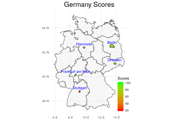
Ok, I think a choropleth would be a good option in this case, here is an example using GDAM data for the polygons.

library(tidyverse)
library(rnaturalearth)

scores <- data.frame(stringsAsFactors = FALSE,
                     NAME_3 = c("Berlin", "Hannover", "Dresden", "Frankfurt am Main", "Stuttgart"),
                     score = c(80, 70, 90, 100, 20))

germany <- ne_states(country = "germany", returnclass = "sf") %>%
    select(name)

# You can download this file from the GDAM site
scored_regions <- readRDS(file = "gadm36_DEU_3_sf.rds") %>% 
    filter(NAME_3 %in% scores$NAME_3) %>% 
    full_join(scores)

ggplot() +
    geom_sf(data = germany, alpha = 0.3) +
    geom_sf(data = scored_regions, aes(fill = score)) +
    geom_sf_text(data = scored_regions, aes(label = NAME_3), nudge_y = 0.3, color = "blue") +
    scale_fill_gradient(low = "red", high = "green") +
    labs(title = "Germany Scores",
         fill = "Scores") +
    theme_minimal() +
    theme(plot.title = element_text(hjust = 0.5, size = 20),
          axis.title = element_blank(),
          plot.background = element_blank(),
          legend.position = c(0.95, 0.20),
          plot.margin = margin(5, 0, 5, 0))

Created on 2019-09-11 by the reprex package (v0.3.0.9000)

1 Like

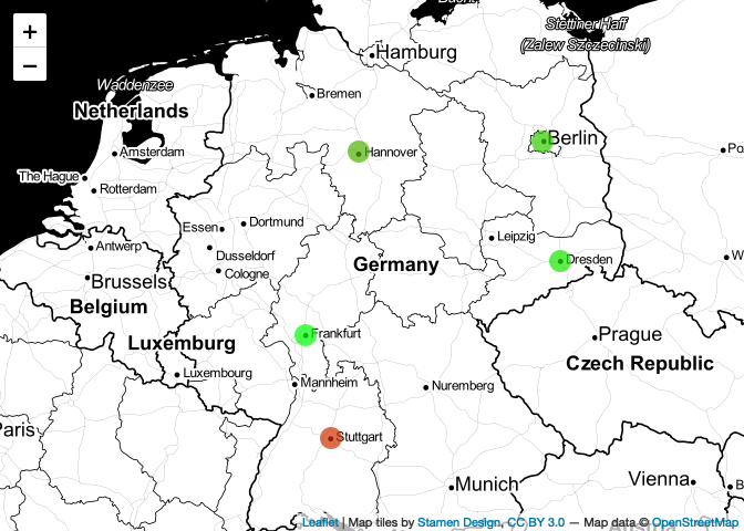
Hi @Slavek. There are many way to plot map in r. The leaflet package is also good for plotting map.

library(tidyverse)
#> Warning: package 'ggplot2' was built under R version 3.4.4
#> Warning: package 'tibble' was built under R version 3.4.3
#> Warning: package 'tidyr' was built under R version 3.4.4
#> Warning: package 'readr' was built under R version 3.4.4
#> Warning: package 'purrr' was built under R version 3.4.4
#> Warning: package 'dplyr' was built under R version 3.4.4
#> Warning: package 'stringr' was built under R version 3.4.4
#> Warning: package 'forcats' was built under R version 3.4.3
library(maps)
#> Warning: package 'maps' was built under R version 3.4.4
#> 
#> Attaching package: 'maps'
#> The following object is masked from 'package:purrr':
#> 
#>     map
library(leaflet)
#> Warning: package 'leaflet' was built under R version 3.4.4

df <- data.frame(stringsAsFactors=FALSE,
                 City = c("Berlin", "Hanover", "Dresden", "Frankfurt", "Stuttgart"),
                 Score = c(80, 70, 90, 100, 20)
)

cites <- world.cities %>%
  as.data.frame() %>%
  filter(name %in% df$City, country.etc == "Germany") %>%
  distinct(name, .keep_all = TRUE) %>%
  left_join(df, by = c("name" = "City"))
#> Warning: package 'bindrcpp' was built under R version 3.4.4

m <- leaflet() %>%
  setView(lng = 10, lat = 51, zoom = 5.5)
m %>%
  addProviderTiles(providers$Stamen.Toner) %>%
  addCircleMarkers(
    data = cites,
    fillColor = ~colorRampPalette(c("red", "green"))(100)[Score],
    stroke = FALSE,
    fillOpacity = 0.7
  )
#> Assuming "long" and "lat" are longitude and latitude, respectively

Created on 2019-09-11 by the reprex package (v0.3.0)

Hope the above can help.

1 Like

@raytong updating your packages should eliminate the warning messages.

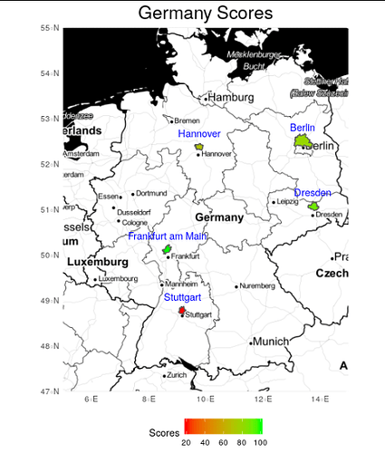
In case you prefer stamen maps style, you can also use them with choropleths using ggplot + ggmap

germany_stamen <- get_stamenmap(bbox = c(left = 5, 
                                    bottom = 47, 
                                    right = 15, 
                                    top = 55),
                           zoom = 6, 
                           maptype = "toner")

ggmap(germany_stamen) +
    geom_sf(data = scored_regions, aes(fill = score), inherit.aes = FALSE) +
    geom_sf_text(data = scored_regions, aes(label = NAME_3), nudge_y = 0.3, color = "blue", inherit.aes = FALSE) +
    scale_fill_gradient(low = "red", high = "green") +
    labs(title = "Germany Scores",
         fill = "Scores") +
    theme_minimal() +
    theme(plot.title = element_text(hjust = 0.5, size = 20),
          axis.title = element_blank(),
          plot.background = element_blank(),
          legend.position = "bottom",
          plot.margin = margin(5, 0, 5, 0))
2 Likes

Thank you. raytong's solution is working but I have a little issue with andresrcs's solution which I actually prefer for this exercise.

Error in gzfile(file, "rb") : cannot open the connection
In addition: Warning message:
In gzfile(file, "rb") :
  cannot open compressed file 'gadm36_DEU_3_sf.rds', probable reason 'No such file or directory'

I looked at the GDAM data and tried other names but the error stays the same.

Maybe its not about the file but a missing package required to have full 'rnaturalearth' functionality?

Can you help please?

Hi @Slavek!

You'll most likely want to download the file from this page and then make sure your code is referencing it using the correct path to the location where you saved the downloaded file.

However, as an illustration, you can also download the file within your code:

url_regions <- "https://biogeo.ucdavis.edu/data/gadm3.6/Rsf/gadm36_DEU_3_sf.rds"
scored_regions <- readRDS(url(url_regions)) %>% 
    filter(NAME_3 %in% scores$NAME_3) %>% 
    full_join(scores)
1 Like

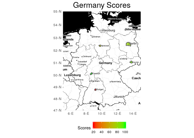
I just have noticed that polygons are not where they should be on the stamen map, there is a small offset. I have found a solution and explanation for this problem on this github issue, here is the example with the solution.

library(tidyverse)
library(ggmap)
library(sf)

scores <- data.frame(stringsAsFactors = FALSE,
                     NAME_3 = c("Berlin", "Hannover", "Dresden", "Frankfurt am Main", "Stuttgart"),
                     score = c(80, 70, 90, 100, 20))

url_regions <- "https://biogeo.ucdavis.edu/data/gadm3.6/Rsf/gadm36_DEU_3_sf.rds"
scored_regions <- readRDS(url(url_regions)) %>% 
    filter(NAME_3 %in% scores$NAME_3) %>% 
    full_join(scores)

germany_stamen <- get_stamenmap(bbox = c(left = 5, 
                                    bottom = 47, 
                                    right = 15, 
                                    top = 55),
                           zoom = 6, 
                           maptype = "toner")

# Define a function to fix the bbox to be in EPSG:3857
ggmap_bbox <- function(map) {
  if (!inherits(map, "ggmap")) stop("map must be a ggmap object")
  # Extract the bounding box (in lat/lon) from the ggmap to a numeric vector, 
  # and set the names to what sf::st_bbox expects:
  map_bbox <- setNames(unlist(attr(map, "bb")), 
                       c("ymin", "xmin", "ymax", "xmax"))
  
  # Coonvert the bbox to an sf polygon, transform it to 3857, 
  # and convert back to a bbox (convoluted, but it works)
  bbox_3857 <- st_bbox(st_transform(st_as_sfc(st_bbox(map_bbox, crs = 4326)), 3857))
  
  # Overwrite the bbox of the ggmap object with the transformed coordinates 
  attr(map, "bb")$ll.lat <- bbox_3857["ymin"]
  attr(map, "bb")$ll.lon <- bbox_3857["xmin"]
  attr(map, "bb")$ur.lat <- bbox_3857["ymax"]
  attr(map, "bb")$ur.lon <- bbox_3857["xmax"]
  map
}

germany_stamen_crs_3857 <- ggmap_bbox(germany_stamen)

ggmap(germany_stamen_crs_3857) +
    coord_sf(crs = st_crs(3857)) +
    geom_sf(data = st_transform(scored_regions, 3857),
            aes(fill = score),
            inherit.aes = FALSE,
            alpha = 0.7) +
    scale_fill_gradient(low = "red", high = "green") +
    labs(title = "Germany Scores",
         fill = "Scores") +
    theme_minimal() +
    theme(plot.title = element_text(hjust = 0.5, size = 20),
          axis.title = element_blank(),
          plot.background = element_blank(),
          legend.position = "bottom",
          plot.margin = margin(5, 0, 5, 0))
2 Likes

Thank you for your solutions. They are great! Easy to use and easy to apply with cities and towns known.

Is it possible to modify these solutions having full address details such as:

data.frame(stringsAsFactors=FALSE,
    Location = c("40476 Düsseldorf", "88276 Berg", "22041 Hamburg",
                 "83536 Gars", "36151 Burghaun"),
       Score = c(66, 55, 85, 62, 67)
)

I cannot find post codes in the map source (https://biogeo.ucdavis.edu/data/gadm3.6/Rsf/gadm36_DEU_3_sf.rds)

Do we need to use completely different solutions?

I think the easiest solution for that would be to extract the city names using a regular expression and leave the codes aside.

This topic was automatically closed 7 days after the last reply. New replies are no longer allowed.