OK @KarmicDreamwork, here you go - the reprex is down at the bottom on my reply. Let me walk you through some of this, first, though.
Problem Space
You've got state and county names, and want to get them on a map. You've gone through a number of spatial packages, and it seems like there are two fundamental issues. The first is that you're not sure exactly what geometry you need and where to get the data, and the second is that you are not sure how to join the geometric data you have been able to get your hands on with your sample data.
Understanding Geometric Data
There are two fundamental ways to represent spatial data (what we often call "shapefiles") in R - sp objects and sf objects. sf objects are my preferred approach because they look and act like data frames that we are used to working with in other contexts.
You have made a couple of references to mapping the longitude and latitude of each county. I suspect the data you've come across represents the centroid of each county i.e. its geometric midpoint. I describe this as the place where you could balance a flat piece of cardboard cut out in the shape of the county on your finger. This is represented as a point on a map.
However, in my experience, most people want the actual outline of the county itself. In this case you, you want polygon data that represent the cutout of the county itself. Polygons are a series of points connected by lines. I'm going to assume this is the type of data you want, but feel free to let me know if you'd rather work with centroids.
Accessing Spatial Data
You've tried out a number of packages that contain some pre-formatted spatial data. I generally suggest getting the actual spatial data rather than some that is pre-processed. Packages like urbnmapr, maps and mapdata contain a limited set of spatial data that is sometimes useful. However, it is better to learn how to access the raw spatial data from the source.
The easiest way to get U.S. spatial data is the tigris package, which allows you to download a variety of common geometric data sets at either a national extent, for a particular state, or for a particular county. These data are not stored within the package like the other tools you've identified. Rather, you download it directly from the U.S. Census Bureau's API. This gives you the widest latitude (pun intended) to use whatever packages you want for mapping, and gives you to the experience to access a variety of spatial data sets and not just want comes packaged within a specific tool like urbnmapr.
Issues With Your Specific Data
You have two sets of spatial references - state names and county names. You've already correctly worked out a major flaw with storing spatial data that way - we repeat county names between states frequently (there are Washington Counties all over the U.S.) and sometimes even within states (Baltimore County and City, for example, are technically both counties, as are St. Louis City and County).
If you download the U.S.-wide county data set from tigris, it will contain county names but not state names. One part of the reprex below therefore involves converting your state names automatically to state FIPS codes (a two digit unique identifier) so that you don't have to do it by hand. We'll use a package called cdlTools to do this.
When we download the county data from tigris, we also have to make one edit - to convert the state FIPS codes to numeric from character so that they match the output we get from the fips(). I also cut down the number of columns in our county data to make it easier to work with, but this of course is optional!
Joining Data
Once we have both data sets prepped and ready to join, we can use dplyr to complete the join. There are two data sets - an x data set and a y one. In the reproducible example below, your sample data are the x data and the county geometric data are the y data. Thus we also list the sample data (and its key variables) first:
sample_joined <- left_join(sample, counties, by =
    c("state.fips" = "STATEFP", "county.name" = "NAME")) %>%
  st_as_sf()
By using two key relationships ("state.fips" = "STATEFP" and "county.name" = "NAME") we can correctly match observations by both county name and state, so that Adams County, Washington is correctly matched with the geometry for that place and Adams County, Colorado is correctly matched with its own geometry.
This will give you a data set with the name number of observations as sample, but each will have the geometric data from counties appended to it. Since our x data are a tibble, we get a nibble out of this. Thus we need to include st_as_sf() after the join to covert our resulting data into an sf object.
If we reversed this, and placed counties as the x data and sample as the y data, we could get resulting object with all of the observations from counties. When a match with sample exists, the sample data will be appended. Otherwise, NA values will be returned. Since counties is already an sf object, you would not need st_as_sf() in this case after the join since the join will return an sf object.
Which data set you list as x and y is a matter of what you want to do with the data next.
Future Data Thoughts
If you continue working with these data, I would suggest using a GEOID that matches the GEOID data present in Census data releases. You may even already have this. It makes the joins easier because GEOID values are always unique and you won't have to worry about Adams County in Washington vs Colorado etc.
Mapping
Since you're using sf objects, you have a bunch of options for mapping. You can use ggplot2, ggmap, tmap, and leaflet just to name a few tools. I like mapview for previewing data and leaflet for web mapping. I teach and use tmap and ggplot2 for static mapping.
Reproducible Example
# dependencies
library(cdlTools)
library(dplyr)
#>
#> Attaching package: 'dplyr'
#> The following objects are masked from 'package:stats':
#>
#> filter, lag
#> The following objects are masked from 'package:base':
#>
#> intersect, setdiff, setequal, union
library(leaflet)
library(tigris)
#> To enable
#> caching of data, set `options(tigris_use_cache = TRUE)` in your R script or .Rprofile.
#>
#> Attaching package: 'tigris'
#> The following object is masked from 'package:graphics':
#>
#> plot
library(sf)
#> Linking to GEOS 3.6.1, GDAL 2.1.3, PROJ 4.9.3
# sample data
sample <- tibble(
state.name = c("South Carolina", "Idaho", "Oklahoma", "Colorado", "Illinois",
"Mississippi", "Ohio", "Pennsylvania", "Washington", "South Carolina"),
county.name = c("Abbeville", "Ada", "Adair", "Adams", "Adams", "Adams", "Adams",
"Adams", "Adams", "Aiken"),
TotalAvgAQI = c(40.8139158576052, 43.1923436041083, 44.8194029850746, 49.606386153387,
38.7736612702366, 43.1960167714885, 32.4834321590513, 40.3827089337176,
26.8103574033552, 37.3312078019505),
TotalAQI1717 = c(NA, 46.5274725274725, 40.4725274725275, 49, 36.9672131147541, NA,
22.8681318681319, 38.1648351648352, 31.1136363636364, 36.7241379310345),
difference = c(NA, 3.33512892336422, -4.34687551254715, -0.606386153387049, -1.80644815548252,
NA, -9.61530029091941, -2.21787376888241, 4.30327896028115, -0.607069870916007))
# convert state names to FIPS codes
sample <- sample %>%
mutate(state.fips = fips(state.name)) %>%
select(state.name, state.fips, everything())
# download counties
counties <- counties(class = "sf")
# subset counties, make fips numeric
counties <- counties %>%
select(STATEFP, NAME) %>%
mutate(STATEFP = as.numeric(STATEFP))
# join sample data with counties
sample_joined <- left_join(sample, counties, by =
c("state.fips" = "STATEFP", "county.name" = "NAME")) %>%
st_as_sf()
#> Warning: Column `state.fips`/`STATEFP` has different attributes on LHS and
#> RHS of join
# leaflet map
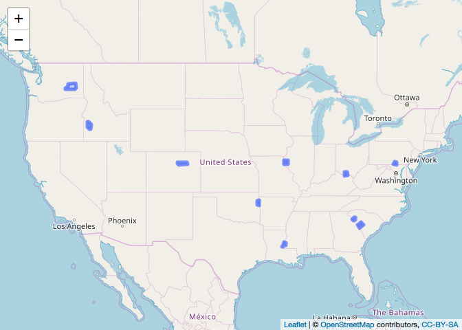
sample_joined %>%
leaflet() %>%
addTiles() %>%
addPolygons()
#> Warning: sf layer has inconsistent datum (+proj=longlat +datum=NAD83 +no_defs).
#> Need '+proj=longlat +datum=WGS84'
Created on 2019-03-24 by the reprex package (v0.2.1)