Loop: difficulty in outputting graphs for each column of a table

Hello everyone,

This is my first time posting on a forum so please feel free to give me advice on how to use it. As far as my level on R is concerned, I have a few basics and I'm trying to improve each day.

My problem : I'm trying to create a loop that allows me to output a graph for each column of a table (for now, I can output graphs but they are empty).

Context / Data: When a subject A moves in a square room, I record the position of the subject in the room (XY) and the activity of cells/neurons (between 50 and 200).

I have 2 sets of data:

  1. The path followed during the experiment (Frame by Frame (one frame=one row of the table), I have access to the X and Y position)
  2. The activity of cells (between 50 and 200 cells, Frame by Frame for each cell activated; 1 = active and 0 = not active)

What I want:
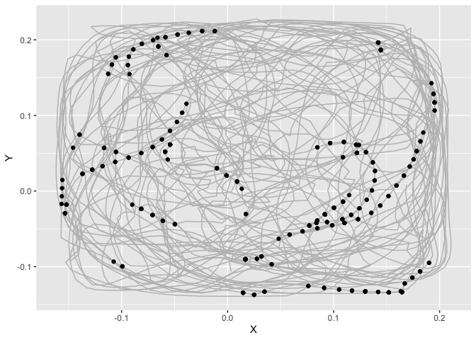
For 1 cell, I want to output an "XY graph that represents the square room" with the path traveled by the subject and overlap the events i.e. place a point when the cell is active (=1)
A map of the activity of the cell in the room

=> Given that I have a large number of cells (therefore a large number of columns in my table). I want to create a loop that automatically outputs the graph / activity map of all my cells.

My progress : I have found a way to plot the graphs of interest for a cell. (Here is the code for 1 cells, N°38)

library(ggplot2)
library(grid)
library(dplyr)
library(knitr)
library(data.table)
library(RColorBrewer)
library(reprex)

palette <- colorRampPalette(c("darkblue", "blue", "lightblue1", "green","yellow", "red", "darkred"))

event <- read.csv2("CaDriftT0.csv",header=T,dec = ",") #Cells event
posdrift <- read.csv2("Raw_dataDriftT0.csv",header=T,dec = ",") #Position
x <- posdrift$X.center
y <- posdrift$Y.center

dtall <- data.table(X=x, Y=y, event) #create  data table X, Y, Time, time sync, C00, C001, C002, ...
dtall <- select(dtall,-Time.s.,-Time.sync.) #Remove 2 columns : Time.s.,-Time.sync.
suball <- subset(dtall, C38 == "1") #If i change Cells Number, i will have the graph and heatmap for this cell -> ==1 select frame where cell was activated

p <- ggplot(data = suball, aes(X,Y))
p + geom_path(data = dtall,aes(X,Y),color = "gray")+ geom_point () #See where are the event on track
image

p + stat_density2d(aes(fill = ..density..), geom = "tile", contour = FALSE, n = 32) + scale_fill_gradientn(colors = palette(10))+ theme_classic() #Heatmap
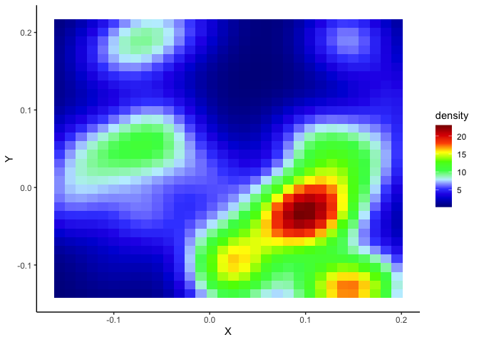
image

I have started to create a loop that repeats the main steps (starting with column 60 to reduce the size of the compilation file). In this loop, my logic is that if I change the column/cell specified in the subset() command, then I change the column/cell at each turn of the loop and the data taken into account in the graphs.
But, when I compiled the document to see what I get: I do get the plot via the X and Y positions of the data.table "dtall", however, the points representing the "1" events in the cell do not appear. Similarly for the heatmap of events, it only creates an empty graph (with the XY axis)

## Loop ## -> I chose 70 at random in order to reduce the number of columns to process

for (i in 70:ncol(dtall)){
  suballo = subset(dtall, i == "1")
  p <- ggplot(data = suballo, aes(X,Y))
  print(p + geom_path(data = dtall,aes(X,Y),color = "gray")+ geom_point ())
  print(p + stat_density2d(aes(fill = ..density..), geom = "tile", contour = FALSE,  n = 16) + scale_fill_gradientn(colors = palette(10))+  theme_classic())
}
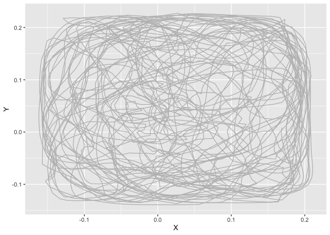
image
image

I am sharing the .csv files on this Github to visualize the data, which I hope is a safe way for you ! GitHub - Anthorhinal/FilesRstudioForum: Csv files

Other information : I don't use data.frame because the length of the columns are different. That's why I chose data.table. I hope this does not cause any problems. Also, I was thinking about the subset()as a problem in the loop.
I thank you in advance for the help you will bring me.

Anthorhinal,
1 Like

There's a lot of good stuff here. But I'm not confident that I can necessarily provide an answer.

One thing that sticks out to me is the data used for the loop, as it does not appear to iterate.

for (i in 70:ncol(dtall)){
  suballo = subset(dtall, i == "1")    
#  ---- The "suballo" looks to be equivelent to the "dtall"; the subset() does not appear to use "i" to manipulate/reshape data.
# ...
# ...
}

I may have some sort of solution.

This reshapes the dtall into a longer format; change values of cell to numeric for iteration

Reshape

dt_all <- dtall
dt_all_long <- unique(
  melt(
    dt_all,
    id.vars = c("x", "y"),
    measure.vars = patterns("^C"),
    variable.name = "cell",
    value.name = "value"
  )[value == 1, .(cell = as.numeric(gsub("[C]", "", cell)), value), .(x, y)]
)

Table output

> dt_all_long
                x         y cell value
   1: -0.14386800 0.0133233    0     1
   2: -0.14386800 0.0133233    4     1
   3: -0.14386800 0.0133233    7     1
   4: -0.14386800 0.0133233   49     1
   5: -0.14386800 0.0133233   75     1
  ---                                 
8341: -0.03421320 0.0962852   75     1
8342: -0.02786510 0.0866554   75     1
8343: -0.01973840 0.0777485   75     1
8344: -0.01094310 0.0704470   75     1
8345: -0.00325129 0.0637158   75     1

Loop

for (i in 0:75) {
  print(
    ggplot(dt_all_long[cell == i], aes(x, y)) +
      geom_path(size = 1, alpha = .25) +
      geom_point() +
      # theme_classic() +
      xlim(-0.25, 0.25) +
      ylim(-0.25, 0.25) +
      ggtitle(paste("Path in Cell", i))
  )
  print(
    ggplot(dt_all_long[cell == i], aes(x, y)) +
      stat_density2d(aes(fill = ..density..), 
                     geom = "tile", 
                     contour = FALSE) +
      scale_fill_gradientn(colors = palette(10)) +
      theme_classic() +
      xlim(-0.25, 0.25) +
      ylim(-0.25, 0.25) +
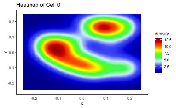
      ggtitle(paste("Heatmap of Cell", i))
  )
}

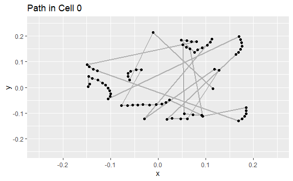
Output

image

image

etc.

2 Likes

Thank you very much for your reactivity and your efficiency! You made me very happy as soon as I saw the different graphics :). I looked at your code most of the afternoon to understand the logic of the different lines. However, I encountered a problem when I ran the code.

library(reshape)
#> 
#> Attachement du package : 'reshape'
#> L'objet suivant est masqué depuis 'package:data.table':
#> 
#>     melt
#> L'objet suivant est masqué depuis 'package:dplyr':
#> 
#>     rename
dt_all <- dtall
dt_all_long <- unique(
  melt(
    dt_all,
    id.vars = c("x", "y"),
    measure.vars = patterns("^C"),
    variable.name = "cell",
    value.name = "value"
  )[value == 1, .(cell = as.numeric(gsub("[C]", "", cell)), value), .(x, y)]
)
#> Error in patterns("^C"): impossible de trouver la fonction "patterns"

Sorry for the French text in the reprex !

« Error in patterns(« ^C») : could not find function « patterns »

I was trying to see what I could do to fix this... but it didn't work, I tried :

  • to not launch other packages
  • Reshape and reshape2 and without both
  • setDT(dt_all)
  • Change the melt() function to melt.data.table(), I got another error.
#> Error in melt.data.table(dt_all, id.vars = c("x", "y"), measure.vars = patterns("^C"), : One or more values in 'id.vars' is invalid.

I tried on a Mac and a windows computer, the problem persists. Maybe you have the solution (do I need an extra package, ...)
Regarding the loop, it's great to see! Although I still couldn't try it out because of the problem I mentioned! I'll try to modify it in order to see the full path of the subject :).

I'll paste what I have used to facilitate it on my end.

I'm determined to get this working for you.

palette <- colorRampPalette(c("darkblue", "blue", "lightblue1", "green","yellow", "red", "darkred"))

# Using fread() to pull from file path
event <- # Cells event
  fread(
    "~/CaDriftT0.csv", # file path
    header = TRUE,
    dec = ","
  ) 

posdrift <- # Position
  fread(
    "~/Raw_dataDriftT0.csv", # file path
    header = TRUE,
    dec = ","
  ) 

# Defining values
x <- posdrift$"X center"
y <- posdrift$"Y center"

# Defining "dtall" and removing time series variables
dtall <- data.table(x, y, event) 
dtall <- select(dtall,-"Time(s)",-"Time(sync)")

## You can also remove these fields in with data.table()
# dtall <- data.table(x, y, event[, `:=` (`Time(s)` = NULL, `Time(sync)` = NULL)])

# Used "dt_all" for better clarity on my end.
dt_all <- dtall
dt_all_long <- unique(
  melt(
    dt_all,
    id.vars = c("x", "y"),
    measure.vars = patterns("^C"),
    variable.name = "cell",
    value.name = "value"
  )[value == 1, .(cell = as.numeric(gsub("[C]", "", cell)), value), .(x, y)]
)

for (i in 0:5) { #reduced to "0:5" for faster response
  print(
    ggplot(dt_all_long[cell == i], aes(x, y)) +
      geom_path(size = 1, alpha = .25) +
      geom_point() +
      # theme_classic() +
      xlim(-0.25, 0.25) +
      ylim(-0.25, 0.25) +
      ggtitle(paste("Path in Cell", i))
  )
  print(
    ggplot(dt_all_long[cell == i], aes(x, y)) +
      stat_density2d(aes(fill = ..density..), 
                     geom = "tile", 
                     contour = FALSE) +
      scale_fill_gradientn(colors = palette(10)) +
      theme_classic() +
      xlim(-0.25, 0.25) +
      ylim(-0.25, 0.25) +
      ggtitle(paste("Heatmap of Cell", i))
  )
}
1 Like

Well, this one works for me! I didn't know the thread() function. I have a few questions to make sure I understand your dt_all_long (). In this line of code you transposed the data to get only the "1"? In this table we get 8345 "1", when checking on the .csv file through " Ctrl+f " (only on the Cxx columns) I found 19527 "1", this means that some data is missing. How can this be explained?

Digging around, I looked at the generation of the data.table on my version and your version. I also noticed a small issue (Cadrift.csv: 12176 rows and Raw_dataDrift.csv: 14988 rows), when we create the dt_all, we have a table of 14988 rows for which "event" values were added for some cells as "1" and others as "0" and not as NA. I also don't know enough about the characteristics of R to explain what is going on here.

In my opinion, these two points cannot be justified by each other :thinking:

As I understand, the x and y values were generated from the posdrift (14988 obs.) and joined to the event (12176 obs.) to create dtall with data.table(x, y, event) .

The two datasets are not synchronous in their times and there's no id or key that we can use to associate between the two with the information currently available.
But that's based on my assumption that there is a relational characteristic between the posdrift and the event sets.

Brief comparrison

join <-
  data.table(
             Pos = posdrift$`Trial time`,
             Eve = c(event$`Time(s)`, rep(NA, 2812))
)
          Pos      Eve
    1:   0.000        0
    2:   0.040 0.049962
    3:   0.080 0.099924
    4:   0.120 0.149886
    5:   0.160 0.199848
   ---                 
14984: 599.852     <NA>
14985: 599.892     <NA>
14986: 599.932     <NA>
14987: 599.972     <NA>
14988: 600.012     <NA>
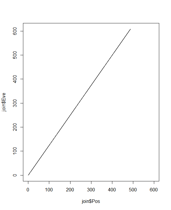
plot(join$Pos, join$Eve, type = "l")

1 Like

Hello,
Thank you for these explanations and I apologize for the delay in answering (I took some disconnected holidays :)). Indeed, in its still very rough data, the times are not synchronized (the frequencies are 20Hz and 25Hz). I plan to apply interpolation formulas in order to find a synchronization! There is still work to be done (especially for statistics to say if the activation in zone is significant)!

1 Like

Identified some issues in my recent reply that invalidates my prior equation.

If time-accuracy is crucial I'd duplicate the experiment (if you are able).

join <-
  data.table(
             Pos = posdrift$`Trial time`,
             Eve = c(event$`Time(s)`, rep(NA, 2812))
)

join[is.na(join)] <- 0

join[, dif := (abs(Pos - as.numeric(Eve)))]

# Shows smaller values preventing alignment through this method
join[, lapply(.SD, diff), .SDcols = 3][, .(dif = as.factor(dif))]

# Rounding by thousandth place
## Increment number (n) in .(dif = round(dif, n)) to see discrepancies
join[, lapply(.SD, diff), .SDcols = 3][, .(dif = round(dif, 2))][, .N, .(dif = as.factor(dif))]

Number (N) of outliers by hundredth

      dif     N
1:   0.01 12175
2: 366.62     1
3:   0.04  2811

Number (N) of outliers by thousandth

       dif     N
1:    0.01 11743
2:   0.009   432
3: 366.617     1
4:    0.04  2711
5:   0.041   100

...

This topic was automatically closed 21 days after the last reply. New replies are no longer allowed.

If you have a query related to it or one of the replies, start a new topic and refer back with a link.