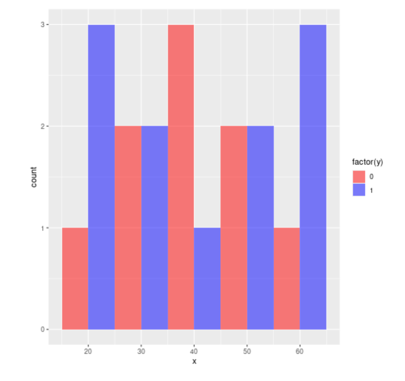
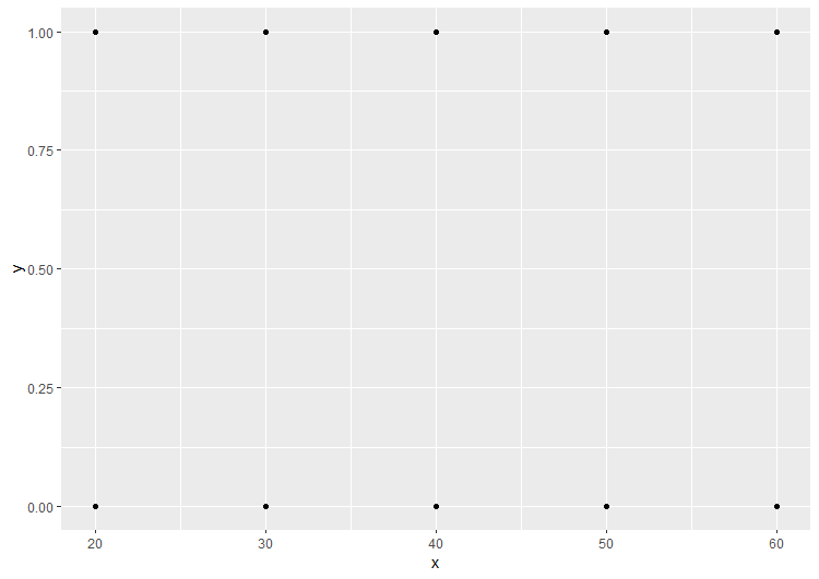
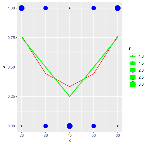
If x is continuous it's hard to see where any glm model will go
# Create the data frame
d <- data.frame(x = c(20,30,30,40,40,40,50,50,60, 20,20,20,30,30,40,50,50,60,60,60),
                y = c(0,0,0,0,0,0,0,0,0,1,1,1,1,1,1,1,1,1,1,1))

# Define the formulas and family arguments
formulas <- list(y ~ x, y ~ I(x^2), y ~ I(sin(x)), y ~ I(sin(x^2)))
families <- list(binomial(link = "logit"),
                 gaussian(link = "identity"),
                 poisson(link = "log"),
                 quasi(link = "identity", variance = "constant"),
                 quasibinomial(link = "logit"),
                 quasipoisson(link = "log"))

# Fit the models and store them in a list
models <- list()
for (f in formulas) {
  for (family in families) {
    model <- glm(f, data = d, family = family)
    models <- append(models, list(model))
  }
}


lapply(models,summary)
#> [[1]]
#>
#> Call:
#> glm(formula = f, family = family, data = d)
#>
#> Coefficients:
#>              Estimate Std. Error z value Pr(>|z|)
#> (Intercept) 2.007e-01  1.348e+00   0.149    0.882
#> x           1.600e-18  3.178e-02   0.000    1.000
#>
#> (Dispersion parameter for binomial family taken to be 1)
#>
#>     Null deviance: 27.526  on 19  degrees of freedom
#> Residual deviance: 27.526  on 18  degrees of freedom
#> AIC: 31.526
#>
#> Number of Fisher Scoring iterations: 3
#>
#>
#> [[2]]
#>
#> Call:
#> glm(formula = f, family = family, data = d)
#>
#> Coefficients:
#>              Estimate Std. Error t value Pr(>|t|)
#> (Intercept) 5.500e-01  3.518e-01   1.563    0.135
#> x           3.806e-19  8.292e-03   0.000    1.000
#>
#> (Dispersion parameter for gaussian family taken to be 0.275)
#>
#>     Null deviance: 4.95  on 19  degrees of freedom
#> Residual deviance: 4.95  on 18  degrees of freedom
#> AIC: 34.831
#>
#> Number of Fisher Scoring iterations: 2
#>
#>
#> [[3]]
#>
#> Call:
#> glm(formula = f, family = family, data = d)
#>
#> Coefficients:
#>               Estimate Std. Error z value Pr(>|z|)
#> (Intercept) -5.978e-01  9.045e-01  -0.661    0.509
#> x            6.096e-18  2.132e-02   0.000    1.000
#>
#> (Dispersion parameter for poisson family taken to be 1)
#>
#>     Null deviance: 13.152  on 19  degrees of freedom
#> Residual deviance: 13.152  on 18  degrees of freedom
#> AIC: 39.152
#>
#> Number of Fisher Scoring iterations: 5
#>
#>
#> [[4]]
#>
#> Call:
#> glm(formula = f, family = family, data = d)
#>
#> Coefficients:
#>              Estimate Std. Error t value Pr(>|t|)
#> (Intercept) 5.500e-01  3.518e-01   1.563    0.135
#> x           3.806e-19  8.292e-03   0.000    1.000
#>
#> (Dispersion parameter for quasi family taken to be 0.275)
#>
#>     Null deviance: 4.95  on 19  degrees of freedom
#> Residual deviance: 4.95  on 18  degrees of freedom
#> AIC: NA
#>
#> Number of Fisher Scoring iterations: 2
#>
#>
#> [[5]]
#>
#> Call:
#> glm(formula = f, family = family, data = d)
#>
#> Coefficients:
#>              Estimate Std. Error t value Pr(>|t|)
#> (Intercept) 2.007e-01  1.421e+00   0.141    0.889
#> x           1.600e-18  3.350e-02   0.000    1.000
#>
#> (Dispersion parameter for quasibinomial family taken to be 1.111123)
#>
#>     Null deviance: 27.526  on 19  degrees of freedom
#> Residual deviance: 27.526  on 18  degrees of freedom
#> AIC: NA
#>
#> Number of Fisher Scoring iterations: 3
#>
#>
#> [[6]]
#>
#> Call:
#> glm(formula = f, family = family, data = d)
#>
#> Coefficients:
#>               Estimate Std. Error t value Pr(>|t|)
#> (Intercept) -5.978e-01  6.396e-01  -0.935    0.362
#> x            6.096e-18  1.508e-02   0.000    1.000
#>
#> (Dispersion parameter for quasipoisson family taken to be 0.5000009)
#>
#>     Null deviance: 13.152  on 19  degrees of freedom
#> Residual deviance: 13.152  on 18  degrees of freedom
#> AIC: NA
#>
#> Number of Fisher Scoring iterations: 5
#>
#>
#> [[7]]
#>
#> Call:
#> glm(formula = f, family = family, data = d)
#>
#> Coefficients:
#>              Estimate Std. Error z value Pr(>|z|)
#> (Intercept) 0.0338639  0.8366883   0.040    0.968
#> I(x^2)      0.0000930  0.0003948   0.236    0.814
#>
#> (Dispersion parameter for binomial family taken to be 1)
#>
#>     Null deviance: 27.526  on 19  degrees of freedom
#> Residual deviance: 27.470  on 18  degrees of freedom
#> AIC: 31.47
#>
#> Number of Fisher Scoring iterations: 4
#>
#>
#> [[8]]
#>
#> Call:
#> glm(formula = f, family = family, data = d)
#>
#> Coefficients:
#>              Estimate Std. Error t value Pr(>|t|)
#> (Intercept) 5.087e-01  2.183e-01   2.330   0.0317 *
#> I(x^2)      2.294e-05  1.024e-04   0.224   0.8253
#> ---
#> Signif. codes:  0 '***' 0.001 '**' 0.01 '*' 0.05 '.' 0.1 ' ' 1
#>
#> (Dispersion parameter for gaussian family taken to be 0.2742355)
#>
#>     Null deviance: 4.9500  on 19  degrees of freedom
#> Residual deviance: 4.9362  on 18  degrees of freedom
#> AIC: 34.775
#>
#> Number of Fisher Scoring iterations: 2
#>
#>
#> [[9]]
#>
#> Call:
#> glm(formula = f, family = family, data = d)
#>
#> Coefficients:
#>               Estimate Std. Error z value Pr(>|z|)
#> (Intercept) -6.734e-01  5.712e-01  -1.179    0.238
#> I(x^2)       4.137e-05  2.616e-04   0.158    0.874
#>
#> (Dispersion parameter for poisson family taken to be 1)
#>
#>     Null deviance: 13.152  on 19  degrees of freedom
#> Residual deviance: 13.128  on 18  degrees of freedom
#> AIC: 39.128
#>
#> Number of Fisher Scoring iterations: 5
#>
#>
#> [[10]]
#>
#> Call:
#> glm(formula = f, family = family, data = d)
#>
#> Coefficients:
#>              Estimate Std. Error t value Pr(>|t|)
#> (Intercept) 5.087e-01  2.183e-01   2.330   0.0317 *
#> I(x^2)      2.294e-05  1.024e-04   0.224   0.8253
#> ---
#> Signif. codes:  0 '***' 0.001 '**' 0.01 '*' 0.05 '.' 0.1 ' ' 1
#>
#> (Dispersion parameter for quasi family taken to be 0.2742355)
#>
#>     Null deviance: 4.9500  on 19  degrees of freedom
#> Residual deviance: 4.9362  on 18  degrees of freedom
#> AIC: NA
#>
#> Number of Fisher Scoring iterations: 2
#>
#>
#> [[11]]
#>
#> Call:
#> glm(formula = f, family = family, data = d)
#>
#> Coefficients:
#>             Estimate Std. Error t value Pr(>|t|)
#> (Intercept) 0.033864   0.881800   0.038    0.970
#> I(x^2)      0.000093   0.000416   0.224    0.826
#>
#> (Dispersion parameter for quasibinomial family taken to be 1.110741)
#>
#>     Null deviance: 27.526  on 19  degrees of freedom
#> Residual deviance: 27.470  on 18  degrees of freedom
#> AIC: NA
#>
#> Number of Fisher Scoring iterations: 4
#>
#>
#> [[12]]
#>
#> Call:
#> glm(formula = f, family = family, data = d)
#>
#> Coefficients:
#>               Estimate Std. Error t value Pr(>|t|)
#> (Intercept) -6.734e-01  4.040e-01  -1.667    0.113
#> I(x^2)       4.137e-05  1.850e-04   0.224    0.826
#>
#> (Dispersion parameter for quasipoisson family taken to be 0.5003108)
#>
#>     Null deviance: 13.152  on 19  degrees of freedom
#> Residual deviance: 13.128  on 18  degrees of freedom
#> AIC: NA
#>
#> Number of Fisher Scoring iterations: 5
#>
#>
#> [[13]]
#>
#> Call:
#> glm(formula = f, family = family, data = d)
#>
#> Coefficients:
#>             Estimate Std. Error z value Pr(>|z|)
#> (Intercept)  0.20207    0.44983   0.449    0.653
#> I(sin(x))   -0.06305    0.63278  -0.100    0.921
#>
#> (Dispersion parameter for binomial family taken to be 1)
#>
#>     Null deviance: 27.526  on 19  degrees of freedom
#> Residual deviance: 27.516  on 18  degrees of freedom
#> AIC: 31.516
#>
#> Number of Fisher Scoring iterations: 3
#>
#>
#> [[14]]
#>
#> Call:
#> glm(formula = f, family = family, data = d)
#>
#> Coefficients:
#>             Estimate Std. Error t value Pr(>|t|)
#> (Intercept)   0.5503     0.1173   4.692 0.000181 ***
#> I(sin(x))    -0.0156     0.1650  -0.095 0.925705
#> ---
#> Signif. codes:  0 '***' 0.001 '**' 0.01 '*' 0.05 '.' 0.1 ' ' 1
#>
#> (Dispersion parameter for gaussian family taken to be 0.2748634)
#>
#>     Null deviance: 4.9500  on 19  degrees of freedom
#> Residual deviance: 4.9475  on 18  degrees of freedom
#> AIC: 34.821
#>
#> Number of Fisher Scoring iterations: 2
#>
#>
#> [[15]]
#>
#> Call:
#> glm(formula = f, family = family, data = d)
#>
#> Coefficients:
#>             Estimate Std. Error z value Pr(>|z|)
#> (Intercept) -0.59746    0.30152  -1.981   0.0475 *
#> I(sin(x))   -0.02837    0.42441  -0.067   0.9467
#> ---
#> Signif. codes:  0 '***' 0.001 '**' 0.01 '*' 0.05 '.' 0.1 ' ' 1
#>
#> (Dispersion parameter for poisson family taken to be 1)
#>
#>     Null deviance: 13.152  on 19  degrees of freedom
#> Residual deviance: 13.148  on 18  degrees of freedom
#> AIC: 39.148
#>
#> Number of Fisher Scoring iterations: 5
#>
#>
#> [[16]]
#>
#> Call:
#> glm(formula = f, family = family, data = d)
#>
#> Coefficients:
#>             Estimate Std. Error t value Pr(>|t|)
#> (Intercept)   0.5503     0.1173   4.692 0.000181 ***
#> I(sin(x))    -0.0156     0.1650  -0.095 0.925705
#> ---
#> Signif. codes:  0 '***' 0.001 '**' 0.01 '*' 0.05 '.' 0.1 ' ' 1
#>
#> (Dispersion parameter for quasi family taken to be 0.2748634)
#>
#>     Null deviance: 4.9500  on 19  degrees of freedom
#> Residual deviance: 4.9475  on 18  degrees of freedom
#> AIC: NA
#>
#> Number of Fisher Scoring iterations: 2
#>
#>
#> [[17]]
#>
#> Call:
#> glm(formula = f, family = family, data = d)
#>
#> Coefficients:
#>             Estimate Std. Error t value Pr(>|t|)
#> (Intercept)  0.20207    0.47416   0.426    0.675
#> I(sin(x))   -0.06305    0.66702  -0.095    0.926
#>
#> (Dispersion parameter for quasibinomial family taken to be 1.111133)
#>
#>     Null deviance: 27.526  on 19  degrees of freedom
#> Residual deviance: 27.516  on 18  degrees of freedom
#> AIC: NA
#>
#> Number of Fisher Scoring iterations: 3
#>
#>
#> [[18]]
#>
#> Call:
#> glm(formula = f, family = family, data = d)
#>
#> Coefficients:
#>             Estimate Std. Error t value Pr(>|t|)
#> (Intercept) -0.59746    0.21321  -2.802   0.0118 *
#> I(sin(x))   -0.02837    0.30010  -0.095   0.9257
#> ---
#> Signif. codes:  0 '***' 0.001 '**' 0.01 '*' 0.05 '.' 0.1 ' ' 1
#>
#> (Dispersion parameter for quasipoisson family taken to be 0.4999959)
#>
#>     Null deviance: 13.152  on 19  degrees of freedom
#> Residual deviance: 13.148  on 18  degrees of freedom
#> AIC: NA
#>
#> Number of Fisher Scoring iterations: 5
#>
#>
#> [[19]]
#>
#> Call:
#> glm(formula = f, family = family, data = d)
#>
#> Coefficients:
#>              Estimate Std. Error z value Pr(>|z|)
#> (Intercept) 0.2008760  0.4939680   0.407    0.684
#> I(sin(x^2)) 0.0006551  0.6539372   0.001    0.999
#>
#> (Dispersion parameter for binomial family taken to be 1)
#>
#>     Null deviance: 27.526  on 19  degrees of freedom
#> Residual deviance: 27.526  on 18  degrees of freedom
#> AIC: 31.526
#>
#> Number of Fisher Scoring iterations: 3
#>
#>
#> [[20]]
#>
#> Call:
#> glm(formula = f, family = family, data = d)
#>
#> Coefficients:
#>              Estimate Std. Error t value Pr(>|t|)
#> (Intercept) 0.5500508  0.1288682   4.268 0.000462 ***
#> I(sin(x^2)) 0.0001621  0.1706006   0.001 0.999252
#> ---
#> Signif. codes:  0 '***' 0.001 '**' 0.01 '*' 0.05 '.' 0.1 ' ' 1
#>
#> (Dispersion parameter for gaussian family taken to be 0.275)
#>
#>     Null deviance: 4.95  on 19  degrees of freedom
#> Residual deviance: 4.95  on 18  degrees of freedom
#> AIC: 34.831
#>
#> Number of Fisher Scoring iterations: 2
#>
#>
#> [[21]]
#>
#> Call:
#> glm(formula = f, family = family, data = d)
#>
#> Coefficients:
#>               Estimate Std. Error z value Pr(>|z|)
#> (Intercept) -0.5977447  0.3313258  -1.804   0.0712 .
#> I(sin(x^2))  0.0002948  0.4386113   0.001   0.9995
#> ---
#> Signif. codes:  0 '***' 0.001 '**' 0.01 '*' 0.05 '.' 0.1 ' ' 1
#>
#> (Dispersion parameter for poisson family taken to be 1)
#>
#>     Null deviance: 13.152  on 19  degrees of freedom
#> Residual deviance: 13.152  on 18  degrees of freedom
#> AIC: 39.152
#>
#> Number of Fisher Scoring iterations: 5
#>
#>
#> [[22]]
#>
#> Call:
#> glm(formula = f, family = family, data = d)
#>
#> Coefficients:
#>              Estimate Std. Error t value Pr(>|t|)
#> (Intercept) 0.5500508  0.1288682   4.268 0.000462 ***
#> I(sin(x^2)) 0.0001621  0.1706006   0.001 0.999252
#> ---
#> Signif. codes:  0 '***' 0.001 '**' 0.01 '*' 0.05 '.' 0.1 ' ' 1
#>
#> (Dispersion parameter for quasi family taken to be 0.275)
#>
#>     Null deviance: 4.95  on 19  degrees of freedom
#> Residual deviance: 4.95  on 18  degrees of freedom
#> AIC: NA
#>
#> Number of Fisher Scoring iterations: 2
#>
#>
#> [[23]]
#>
#> Call:
#> glm(formula = f, family = family, data = d)
#>
#> Coefficients:
#>              Estimate Std. Error t value Pr(>|t|)
#> (Intercept) 0.2008760  0.5206907   0.386    0.704
#> I(sin(x^2)) 0.0006551  0.6893139   0.001    0.999
#>
#> (Dispersion parameter for quasibinomial family taken to be 1.111123)
#>
#>     Null deviance: 27.526  on 19  degrees of freedom
#> Residual deviance: 27.526  on 18  degrees of freedom
#> AIC: NA
#>
#> Number of Fisher Scoring iterations: 3
#>
#>
#> [[24]]
#>
#> Call:
#> glm(formula = f, family = family, data = d)
#>
#> Coefficients:
#>               Estimate Std. Error t value Pr(>|t|)
#> (Intercept) -0.5977447  0.2342830  -2.551    0.020 *
#> I(sin(x^2))  0.0002948  0.3101453   0.001    0.999
#> ---
#> Signif. codes:  0 '***' 0.001 '**' 0.01 '*' 0.05 '.' 0.1 ' ' 1
#>
#> (Dispersion parameter for quasipoisson family taken to be 0.5000009)
#>
#>     Null deviance: 13.152  on 19  degrees of freedom
#> Residual deviance: 13.152  on 18  degrees of freedom
#> AIC: NA
#>
#> Number of Fisher Scoring iterations: 5
Created on 2023-07-09 with reprex v2.0.2