@JohnMount
Hello John,
Question 1:
> glm_model <- glm(down_train$Class~.,data = down_train, family = binomial)
Warning message:
glm.fit: fitted probabilities numerically 0 or 1 occurred
> summary(glm_model)

Call:
glm(formula = down_train$Class ~ ., family = binomial, data = down_train)

Deviance Residuals:
    Min       1Q   Median       3Q      Max
-2.1399  -1.0367   0.2300   0.9208   8.4904

Coefficients:
                                         Estimate  Std. Error  z value             Pr(>|z|)
(Intercept)                           -11.4108728  23.4467343   -0.487              0.62649
cust_prog_levelC                        1.1169289   0.1379501    8.097 0.000000000000000565 ***
cust_prog_levelD                        0.9901193   0.1298182    7.627 0.000000000000024034 ***
cust_prog_levelE                        1.1544305   0.1338535    8.625 < 0.0000000000000002 ***
cust_prog_levelG                        0.9318156   0.1293693    7.203 0.000000000000590075 ***
cust_prog_levelI                        1.2254934   0.1324209    9.255 < 0.0000000000000002 ***
cust_prog_levelL                        1.2905412   0.1296241    9.956 < 0.0000000000000002 ***
cust_prog_levelM                        0.9916104   0.3064315    3.236              0.00121 **
cust_prog_levelN                        1.2756395   0.1293191    9.864 < 0.0000000000000002 ***
cust_prog_levelP                        0.9498830   0.1293275    7.345 0.000000000000206089 ***
cust_prog_levelR                        0.7728894   0.2732953    2.828              0.00468 **
cust_prog_levelS                        0.9850813   0.1294868    7.608 0.000000000000027928 ***
cust_prog_levelX                        1.7231817   0.3874403    4.448 0.000008683257380494 ***
cust_prog_levelZ                        2.2222995   0.1342246   16.557 < 0.0000000000000002 ***
CUST_REGION_DESCRMOUNTAIN WEST REGION  11.0671194  23.4463814    0.472              0.63691
CUST_REGION_DESCRNORTH CENTRAL REGION  11.2638726  23.4463804    0.480              0.63094
CUST_REGION_DESCRNORTH EAST REGION     11.3171832  23.4463806    0.483              0.62932
CUST_REGION_DESCROHIO VALLEY REGION    11.3389408  23.4463811    0.484              0.62866
CUST_REGION_DESCRSOUTH CENTRAL REGION  11.2946499  23.4463802    0.482              0.63000
CUST_REGION_DESCRSOUTH EAST REGION     11.3990264  23.4463799    0.486              0.62684
CUST_REGION_DESCRWESTERN REGION        11.1147124  23.4463816    0.474              0.63547
Sales                                  -0.0107124   0.0000521 -205.598 < 0.0000000000000002 ***
---
Signif. codes:  0 ‘***’ 0.001 ‘**’ 0.01 ‘*’ 0.05 ‘.’ 0.1 ‘ ’ 1

(Dispersion parameter for binomial family taken to be 1)

    Null deviance: 522966  on 377239  degrees of freedom
Residual deviance: 431903  on 377218  degrees of freedom
AIC: 431947

Number of Fisher Scoring iterations: 9
So the summary() give me this result and there are quite a few estimates with standard errors exceed 23. So can I assume the warning message "glm.fit: fitted probabilities numerically 0 or 1 occurred" explains for this large number? I am asking this question because the other standard errors are small and those mentioned above are so so large, so I am curious why!
Question 2: I took your advice and used glmnet() method
>xfactors<-model.matrix(Class ~ CUST_REGION_DESCR + cust_prog_level,data=down_train)[,-1]
>x = as.matrix(data.frame(down_train$Sales,xfactors))
>glmmod = glmnet(x,y=as.factor(down_train$Class),alpha=1,family='binomial')
> summary(glmmod)
           Length Class     Mode
a0           60   -none-    numeric
beta       1260   dgCMatrix S4
df           60   -none-    numeric
dim           2   -none-    numeric
lambda       60   -none-    numeric
dev.ratio    60   -none-    numeric
nulldev       1   -none-    numeric
npasses       1   -none-    numeric
jerr          1   -none-    numeric
offset        1   -none-    logical
classnames    2   -none-    character
call          5   -none-    call
nobs          1   -none-    numeric
What does the result tell me?
One article says that:
if you take logarithm on both side of the below equation,
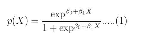
you will get:
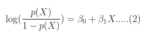
The quantity on the left is the logarithm of the odds. So, the model is a linear regression of the log-odds, sometimes called logit, and hence the name logistic.
Since I have more than one regressor(Sales, cust_program_level, CUST_REGION_DESCR), I assume I will have beta_0, beta_1, beta_2 or something like that.
Should the explanation for summary(glmmod) be focused on whether we have some estimates for those betas just as summary() for a linear regression model?
Thank you!