Linear Regression on Gini Coefficient and Other Bounded Dependant Variables

The Gini Coefficient

The Gini Coefficient is a measure of equality that ranges from 0 (perfect equality) to 1 (a single entity has 100% of some quantity). In a closed post, I suggested that because Gini was a continuous variable, capable of taking on any value between 0 and 1, ordinary least square linear regression would be a good place to start. (Although if it were binary 0 or 1, logistic regression using the binomial family would be required.)

A sidebar

@Yarnabrina and I had a message discussion whether a Gini observation of exactly 0 or exactly 1 would generate a correlation of -Inf or +Inf and, more generally, whether it is guaranteed that predicted results will be bounded by the interval of the dependent variable.

I made the argument from practicality -- the low probability of occurrence justifies starting with the assumption that the data don't contain values of exactly 0 or 1.

A toy model

dat <- runif(1000000)
x <- sample(dat, 1000)
y <- sample(dat, 1000) * sample(dat,1000) * 10
head(x)
mod <- lm(x ~ y)
summary(mod)
## 
## Call:
## lm(formula = x ~ y)
## 
## Residuals:
##      Min       1Q   Median       3Q      Max 
## -0.50109 -0.23728 -0.00731  0.23897  0.51709 
## 
## Coefficients:
##             Estimate Std. Error t value Pr(>|t|)    
## (Intercept) 0.477383   0.013655  34.959   <2e-16 ***
## y           0.004134   0.004059   1.018    0.309    
## ---
## Signif. codes:  0 '***' 0.001 '**' 0.01 '*' 0.05 '.' 0.1 ' ' 1
## 
## Residual standard error: 0.2856 on 998 degrees of freedom
## Multiple R-squared:  0.001038,   Adjusted R-squared:  3.698e-05 
## F-statistic: 1.037 on 1 and 998 DF,  p-value: 0.3088

This is exactly what we would expect to see in regressing a random dependent variable on a random independent variable almost all the time. The intercept is near 0.5 and the coefficient near zero.

A toy pathological case

Now let's see if introducing 0 and 1 into x & y produces any different result

dat <- runif(1000000)
x <- sample(dat, 1000)
x <- c(x,0,1)
y <- sample(dat, 1000) * sample(dat,1000) * 10
y <- c(y,0,1)
mod <- lm(x ~ y)
summary(mod)
## 
## Call:
## lm(formula = x ~ y)
## 
## Residuals:
##      Min       1Q   Median       3Q      Max 
## -0.50373 -0.25385 -0.00786  0.26139  0.51217 
## 
## Coefficients:
##             Estimate Std. Error t value Pr(>|t|)    
## (Intercept) 0.484740   0.013746  35.265   <2e-16 ***
## y           0.003093   0.004028   0.768    0.443    
## ---
## Signif. codes:  0 '***' 0.001 '**' 0.01 '*' 0.05 '.' 0.1 ' ' 1
## 
## Residual standard error: 0.2893 on 1000 degrees of freedom
## Multiple R-squared:  0.0005895,  Adjusted R-squared:  -0.0004099 
## F-statistic: 0.5898 on 1 and 1000 DF,  p-value: 0.4427

No substantive difference is visible.

Are OLS predictions theoretically always within the bounds of the dependant variable?

Peter Dalgaard, Introductory Statistics with R

The linear regression model is provided by

y_i = \alpha + \beta x_i + \epsilon_i

in which the \epsilon_i are assumed independent an N(0,\sigma^2). The nonrandom part of the equation describes the y_i as lying on a straight line. The slope of the line (the regression coefficient) is \beta, the increase per unit change in x. The line intersects the y axis at the intercept \alpha.

at 109.

He then goes on to explain that the method of least squares can be used to estimate \alpha, \beta, \sigma^2 by choosing \alpha, \beta to minimize the sum of squared residuals.

Even if max(x) is paired with max(y) in the data and y \gg x, the residual is still measured relative to the slope, which terminates at max(x) because \ni x > max(x).

I don't see any way of falsifying that conclusion, but my formal training is limited and I invite criticism.
1 Like

Hi, I am not sure regarding what you and @Yarnabrina discussed, but certainly, a single 1 or 0 can generate a confidence interval beyond the boundaries of the dependent variable (with bounded parameters, is is certainly a common issue, i.e. like when estimating survival or transition probabilities and the actual value is close to the edge of the interval). That's a toy example, where y is generated in the interval (0,1) and have added just one 1.

set.seed(20221)
x <- rnorm(100, 30, 6)
y <- c(runif(99),1)
fitted <- summary(lm(y~x))
## upper confidence interval limit:
fitted$coefficients[[1]] + qnorm(.975)*fitted$coefficients[[3]]
[1] 1.093774

The values for the simulation has been choosen completely at random, and for some simulations, it worked and for others like the one i pasted, gave a upper limited beyond the maximum. that's mostly data dependent, but it can certainly happen.

hope it helps to add some to the discussion
cheers

Edit. I have realized that I did my toy example in R version 3.5.'something', at least not R 3.6. Due to the changes on the RNG introduced in R 3.6.X, it may or not gives the expected behavior of having the upper 95% CI beyond the boundary of the parameter...

1 Like

I'd like to refer to one more related thread here, where I suggested my approach (I haven't searched earlier, but now it seems similar to the links I shared below). Actually, this is where Richard pointed out that if sample values are exactly on the boundaries, we'll be in problem. Of course, he is right, but it happens with probability 0. But I understand that the model should be foolproof, and hence there must be a better way.

Regarding linear regression, I think the main problem is that one can't guarantee that the predictions will be in a certain range, as Fernando pointed out. I haven't tried to reproduce it, but it's a line, right? So, unless it's parallel to x-axis (which does not happen, and probability of happening is 0), it'll cross the bound in the y-axis certainly.

[You may have covered this point in the last part of the thread, I didn't really follow it. I didn't understand how slope terminates somewhere. What do you mean by \ni? I didn't get which set contains what x? (Or, is it \exists?)]

Also, it seems to me that the assumptions of linear regression may not be satisfied in this case. Also, the assumption of homoscedasticity is probably not going to be satisfied. As @whuber suggested in the shared link below, the random components corresponding to the Gini coefficients in the boundary region (both 0 and 1 end) are unlikely to have same extent of variation as the ones corresponding to Gini values in the middle region (close to 0.5).

Here are the two relevant links:

https://stats.idre.ucla.edu/stata/faq/how-does-one-do-regression-when-the-dependent-variable-is-a-proportion/

1 Like

Thanks for the insight regarding confidence intervals. That's a separate issue that we hadn't been discussing.

I'd need to do some digging, but I think OLS depends on the assumption that the residuals are normally distributed, which they will be in our toy examples only by chance. The 95% bound is calculate on the mean ± 2z. There is perhaps over conservative and can exceed the defined bounds on the mean (the mean of 0..1 must necessarily be $0 <= \mu <= 1).

1 Like

I'll take this in parts. Thanks, of course you're right, I meant \nexists rather than \notin, not exists rather than not in. I have forgotten more of my 1969 set theory course than I thought.

I made a poor choice of variable names out of the gate, lets switch my x & y to your y & x.

The logit approach is something I'll have to come back to.

I haven't assumed that x is is bounded. It is of course in my second toy example. But it's hard to think of any x predictor that is unbounded. It's not possible to observe infinity, you can only define it. I'm no physicist, but I can't think of any physical attribute that is unbounded (e.g., even c, the speed of light, has an upper bound). My gut feeling is that if you wanted an x to be arbitrarily large, you couldn't use OLS.

In my first toy example the slope is very close to flat, and I'm confident that the mean of a sufficiently large number of Monte Carlo iterations would convert toward x = 0.5y.

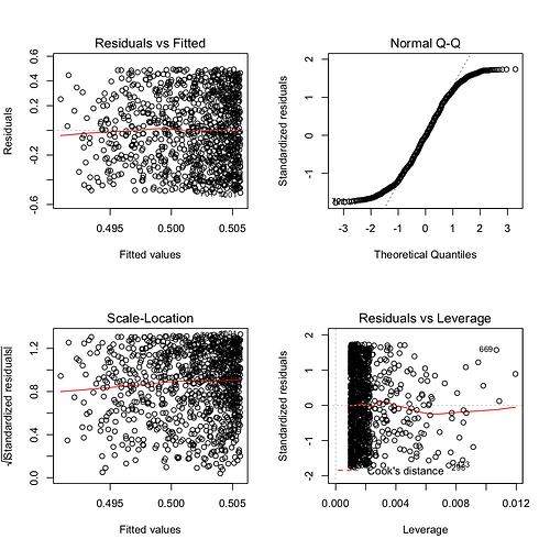
@whuber is correct about the residuals, which are fat tailed on both ends, as shown in the attached plot, and it would be surprising if random $x_i$s would ever satisfy the linear regression requirements. In the absence of any real data to compare observed GINIs to, I don't have any better way to illustrate my origination proposition: when you have continuous dependent variables OLS is a good place to start.

I'll also take a look at the link and comment separately.

Thanks for advancing the ball @Yarnabrina!

1 Like

This topic was automatically closed 21 days after the last reply. New replies are no longer allowed.