First, a general note: normality tests are bad in general, and should probably never be used. This is because in real life, data is never perfectly normal, so if you have a huge sample size, you can always reject the Null hypothesis that your data is normal. On the other hand, if your sample size is too small, you'll fail to reject the Null, even when its distribution is very clearly not normal. So, in a way, the normality tests are more a kind of sample size tests.
In addition, by design, statistical tests are making it hard to reject the Null, and default to accepting it, so a failure to reject the Null is typically not a conclusive result.
That being said, in your situation the easiest might be to try with some fake data.
datos <- c(23,34,45,65,54,32,23,43,54,67,87,65,45,34,54)
set.seed(123)
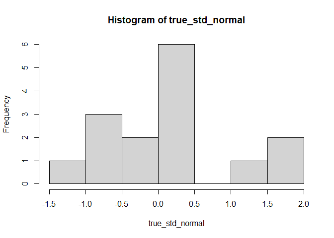
We start with a standard Gaussian distribution, i.e. with mean 0 and sd 1:
true_std_normal <- rnorm(length(datos), mean = 0, sd = 1)

hist(true_std_normal)
qqnorm(true_std_normal)
qqline(true_std_normal)
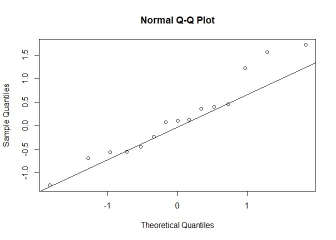
ks.test(x = true_std_normal, pnorm)
#>
#>  Exact one-sample Kolmogorov-Smirnov test
#>
#> data:  true_std_normal
#> D = 0.17942, p-value = 0.6557
#> alternative hypothesis: two-sided
Unsurprisingly, the test fails to reject the Null: we can't say this data is not normal.
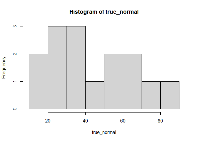
Now, we can try with a normal distribution that is not standard, with a mean and sd that are the same as datos:
true_normal <- rnorm(length(datos), mean = mean(datos), sd = sd(datos))

hist(true_normal)
qqnorm(true_normal)
qqline(true_normal)
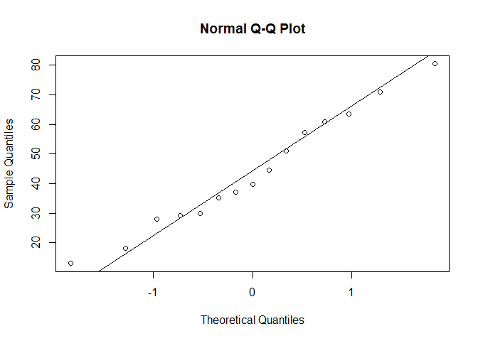
ks.test(x = true_normal, pnorm)
#>
#> 	Exact one-sample Kolmogorov-Smirnov test
#>
#> data:  true_normal
#> D = 1, p-value < 2.2e-16
#> alternative hypothesis: two-sided
So if we test it against a standard distribution, the KS test rejects the Null: the data in true_normal is not compatible with a standard Gaussian. Hence, we want to test it against a non-standard Gaussian, so we need to specify the mean and sd of the theoretical distribution to fit against. We can look at ?ks.test
ks.test(x, y, ...)
Arguments
x a numeric vector of data values.
y either a numeric vector of data values, or a character string naming a cumulative distribution function or an actual cumulative distribution function such as pnorm.
... for the default method, parameters of the distribution specified (as a character string) by y. Otherwise, further arguments to be passed to or from methods.
Thus, we can pass true_normal as x, and pnorm as y, but then we need to add some parameters in .... Let's look at ?pnorm
pnorm(q, mean = 0, sd = 1, lower.tail = TRUE, log.p = FALSE)
So for pnorm(), if we don't specify them, by default mean = 0 and sd = 1, i.e. by default it uses a standard normal. In our case, we want to choose the parameters mean and sd, so we can specify them in the ... of ks.test() and they will be passed on to pnorm().
ks.test(x = true_normal, pnorm, mean(datos), sd(datos))
#>
#>  Exact one-sample Kolmogorov-Smirnov test
#>
#> data:  true_normal
#> D = 0.21515, p-value = 0.4309
#> alternative hypothesis: two-sided
And we fail to reject the Null: our data is compatible with a Normal distribution with the provided mean and sd.
Note that in ... you can pass any argument that pnorm() understands, so for example this is a valid call:
ks.test(x = true_normal, pnorm, lower.tail = FALSE)
But that will fail:
ks.test(x = true_normal, pnorm, wrong_argument = FALSE)
#> Error in y(sort(x), ...) : unused argument (wrong_argument = FALSE)
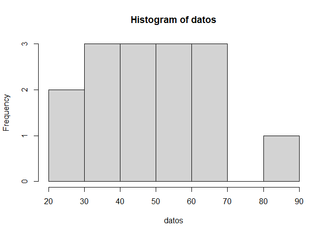
Finally we can look at datos itself:
hist(datos)
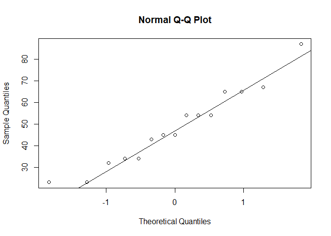
qqnorm(datos)
qqline(datos)
ks.test(x = datos, pnorm)
#>
#> 	Asymptotic one-sample Kolmogorov-Smirnov test
#>
#> data:  datos
#> D = 1, p-value = 1.872e-13
#> alternative hypothesis: two-sided
#>
#> Warning message:
#> In ks.test.default(x = datos, pnorm) :
#>   ties should not be present for the Kolmogorov-Smirnov test


ks.test(x = datos, pnorm, mean(datos), sd(datos))
#> Warning in ks.test.default(x = datos, pnorm, mean(datos), sd(datos)): ties
#> should not be present for the Kolmogorov-Smirnov test
#>
#>  Asymptotic one-sample Kolmogorov-Smirnov test
#>
#> data:  datos
#> D = 0.12114, p-value = 0.9803
#> alternative hypothesis: two-sided
Thus the Null is rejected when comparing to a standard Gaussian, but not rejected when comparing to our non-standard Gaussian.
To come back to my initial point, the latter just means that datos is not extremely different from that non-standard normal distribution, but doesn't mean it's necessarily normal: we have a pretty small sample size here, maybe we just fail to detect the non-normality. The Q-Q plot is much more convincing in that case.
Also of note, we used the data to choose the mean(datos) and sd(datos) to which we are comparing the data. In a way, we "cheated", so the p-value has more than 5% chance of being below 0.05 even when the Null is true.