JAGS: Why my Bayesian model fails to converge?

I'm working on a Bayesian model and stumbled upon some convergence problems. I am sure that I am making a silly mistake, as I have little formal background in Math. Still, I can't identify the problem so I cannot solve it.

Basically, I am sanity-checking the model by applying it to simulated data, so I can compare with "true" values, before I use actual data. My model was designed to be applied to experiments in Psychophysics. Basically, subjects are presented with a series of four physical properties (named x1, x2, x3, x4). Then, they produce a response that combines such properties. However, in this combination they will give more weight to some properties (e.g., A) than to others. The model should take the responses from the whole sample of participants (one response by participant), and estimate the four coefficients that weight the four observations (Psi1, Psi2, Psi3, and Psi4). To ensure you understand me, this is the program that simulates the data in R:

set.seed(40) #This makes the example reproducible...
psi <- runif(4, 0, 1) #This creates a random set of 4 coefficients between 0 and 1.
x <- c(20, 4, 2, 10) #Vector with the 4 physical properties to be learned
combinedX <-   ((psi[1]*x[1])/((psi[1]*x[1])+(psi[2]*x[2]))) - ((psi[3]*x[3])/((psi[3]*x[3])+(psi[4]*x[4]))) 
#This combination rule is a weighted version of Cramer's Phi coefficient of association. Each property x (x[1], x[2], x[3], x[4]) is multiplied by the corresponding coefficient stored in the vector psi.

n <- 50 #I want to simulate 50 data
data <- rnorm(n, combinedX, 0.1) #And they are obtained from a normal distribution with mean combinedX.

I want now to submit these simulated data to a Bayesian model in JAGS that should take the data vector, and output an estimation of the four coefficients.

model{
  psi1 ~ dbeta(1,1)
  psi2 ~ dbeta(1,1)
  psi3 ~ dbeta(1,1)
  psi4 ~ dbeta(1,1)
  predx <- ((psi1*x[1])/ ((psi1*x[1])+(psi2*x[2]))) - ((psi3*x[3])/((psi3*x[3])+(psi4*x[4])))
  sigma <- exp(log_sigma)
  log_sigma ~dunif(-10, 10)

  for(i in 1:n){
    data[i] ~ dnorm(predx, sigma)
  }
}

So, basically, the model only assumes that data come from a normal distribution with mean "predx", which is obtained by combining the four Xs and the four psis.

Good. When I run this model, I obtain nonsensical results most of the times, and often detect problems of convergence, chains that do not mix, extremely flat posteriors (maximal uncertainty), or estimations very different from the actual values...

I suspect two reasons for this behavior:
-Autocorrelation. But, how to solve it?
-The problem is ill-defined: we have too many free parameters (4) to be estimated from data.

Any idea as to what to do with this model?
Thank you in advance.

I am absolutely not an expert on mcmc calculations, so take this as advice from a novice.

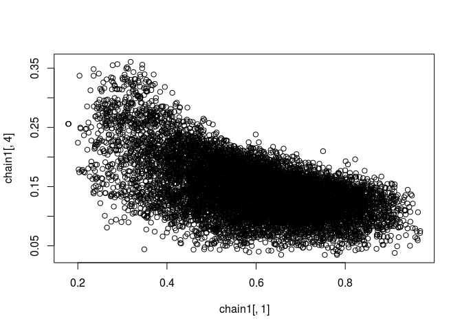
I think you are correct that there are more parameters than can be estimated from the data. I ran the data and model you provided (changing the variable name data to dataM so that it would compile) and the parameter predx is fairly precisely estimated to be 0.26 but the psiX parameters are poorly estimated with a small number of effective samples. Looking at the calculation of predx, if psi1 is anywhere near 1, say above 0.5, then the first part of the predx calculation, involving psi1 and psi2, will give a number well above 0.26. This will force psi4 to be small so that the subtraction can produce the correct predx. If psi1 is small, then the first part of the calculation can be near 0.26 and psi4 must be large to keep the final value correct. This effect can be seen by plotting psi4 vs psi1.

I tried putting a somewhat more "informed" priors on psi1 and psi4, using dbeta(8,4) and dbeta(4,8) so that psi1 will tend to stay high and psi4 will stay low. This improved the result significantly, though the effective number of steps are still pretty low.I am not saying that adjusting the priors is the correct thing to do; you would need to have a reason other than preferring the result to do that. I only used it as an illustration of how the posterior changes as a result.

Of course, psi2 and psi3 also have some effect, though the lower values of x[2] and x[3] decrease their importance.

I hope that helps some.

In the plots below, psi1 is on the x axis and psi4 is on the y axis.

library(rjags)
#> Loading required package: coda
#> Linked to JAGS 4.2.0
#> Loaded modules: basemod,bugs
library(runjags)
set.seed(40) #This makes the example reproducible...
psi <- runif(4, 0, 1) #This creates a random set of 4 coefficients between 0 and 1.
x <- c(20, 4, 2, 10) #Vector with the 4 physical properties to be learned
combinedX <-   ((psi[1]*x[1])/((psi[1]*x[1])+(psi[2]*x[2]))) - ((psi[3]*x[3])/((psi[3]*x[3])+(psi[4]*x[4]))) 
#This combination rule is a weighted version of Cramer's Phi coefficient of association. Each property x (x[1], x[2], x[3], x[4]) is multiplied by the corresponding coefficient stored in the vector psi.

n <- 50 #I want to simulate 50 data
data <- rnorm(n, combinedX, 0.1) #And they are obtained from a normal distribution with mean combinedX.

dataList <- list( dataM = data, n = n, x = x) 
MODEL <- "
model{
  psi1 ~ dbeta(1,1)
  psi2 ~ dbeta(1,1)
  psi3 ~ dbeta(1,1)
  psi4 ~ dbeta(1,1)
  predx <- ((psi1*x[1])/ ((psi1*x[1])+(psi2*x[2]))) - ((psi3*x[3])/((psi3*x[3])+(psi4*x[4])))
  sigma <- exp(log_sigma)
  log_sigma ~ dunif(-10, 10)

  for ( i in 1:n ) {dataM[i] ~ dnorm(predx, sigma)}
}
"
parameters <- c("psi1", "psi2", "psi3", "psi4", "predx", "sigma")
runJagsOut <- run.jags(model =MODEL, monitor = parameters, data = dataList, n.chains = 3)
#> Warning: No initial values were provided - JAGS will use the same initial
#> values for all chains
#> Compiling rjags model...
#> Calling the simulation using the rjags method...
#> Adapting the model for 1000 iterations...
#> Burning in the model for 4000 iterations...
#> Running the model for 10000 iterations...
#> Simulation complete
#> Calculating summary statistics...
#> Calculating the Gelman-Rubin statistic for 6 variables....
#> Finished running the simulation
summary(runJagsOut)[,c("Mean", "SSeff", "psrf")]
#>             Mean SSeff     psrf
#> psi1   0.2275432    83 1.049747
#> psi2   0.6357897   304 1.008065
#> psi3   0.5602133   340 1.002093
#> psi4   0.4120071   120 1.015010
#> predx  0.2571260 29180 1.000068
#> sigma 86.9197751 18670 1.000146
codaSamples = as.mcmc.list( runJagsOut )
chain1 <- codaSamples[[1]]
chain1 <- as.matrix(chain1)
plot(chain1[,1], chain1[,4])


MODEL <- "
model{
  psi1 ~ dbeta(8,4)
  psi2 ~ dbeta(1,1)
  psi3 ~ dbeta(1,1)
  psi4 ~ dbeta(4,8)
  predx <- ((psi1*x[1])/ ((psi1*x[1])+(psi2*x[2]))) - ((psi3*x[3])/((psi3*x[3])+(psi4*x[4])))
  sigma <- exp(log_sigma)
  log_sigma ~ dunif(-10, 10)

  for ( i in 1:n ) {dataM[i] ~ dnorm(predx, sigma)}
}
"

runJagsOut <- run.jags(model =MODEL, monitor = parameters, data = dataList, n.chains = 3)
#> Warning: No initial values were provided - JAGS will use the same initial
#> values for all chains
#> Compiling rjags model...
#> Calling the simulation using the rjags method...
#> Adapting the model for 1000 iterations...
#> Burning in the model for 4000 iterations...
#> Running the model for 10000 iterations...
#> Simulation complete
#> Calculating summary statistics...
#> Calculating the Gelman-Rubin statistic for 6 variables....
#> Finished running the simulation
summary(runJagsOut)[,c("Mean", "SSeff", "psrf")]
#>             Mean SSeff     psrf
#> psi1   0.6082240  1250 1.002243
#> psi2   0.7204599   715 1.002359
#> psi3   0.8067073   749 1.002307
#> psi4   0.1401493   384 1.011632
#> predx  0.2591560 29241 1.000005
#> sigma 87.0936436 18079 1.000138
codaSamples = as.mcmc.list( runJagsOut )
chain1 <- codaSamples[[1]]
chain1 <- as.matrix(chain1)
plot(chain1[,1], chain1[,4])

Created on 2020-03-13 by the reprex package (v0.2.1)

1 Like

Thank you for your help!

From my limited understanding of these modeling techniques, I still don’t get why four parameters cannot be estimated from a sample of 50 data. I’ve seen more complex models (hierarchical, with many free parameters…)

However, I think that part of the problem is that the parameters are correlated, so this would be more or less specific to my modeling situation. This is somewhat clear from your exposition: if psi1 is high, then psi4 must be small. And your plots seem to confirm this idea.

I don’t know if this has some solution. Perhaps I can rethink the model so that there is a latent node that prevents the correlation?

Would you think that the problem is unsolvable?
Thanks again for your work.

I did not express myself well when I implied that four parameters cannot be estimated from 50 data points. What I meant is that the psiX parameters cannot be efficiently estimated from the data because the data are consistent with any psiX values that produce a predx of 0.26. There is no basis on which to choose the psiX values other than their combined value if you use flat priors. If you run the chains long enough, they will eventually map out all of the psiX values that work and be well mixed but that might take an impractical amount of time. When using real data that does not have as well defined a relationship to predx and sigma as the synthetic data, I can imagine that the psiX values are even less restricted.

Not knowing anything about your application, I can't suggest how best to proceed. If you really have no idea of what the values of the psiX are, so the you cannot tighten the priors, it seems it will be very hard to learn much about their values. predx and sigma can be estimated well. Are those less interesting than the psiX?

By the way, the parameters of dnorm in JAGS are the mean and precision (the inverse of the variance), so sigma is not the standard deviation. You may well know that but calling the precision sigma made me think you might have missed that detail.

Again, I am no expert. Someone may come along with a simple solution.

1 Like

This topic was automatically closed 21 days after the last reply. New replies are no longer allowed.