Iterate plot function over columns and add column name as title

HABSaremyjam · December 5, 2022, 8:39pm

Hello,

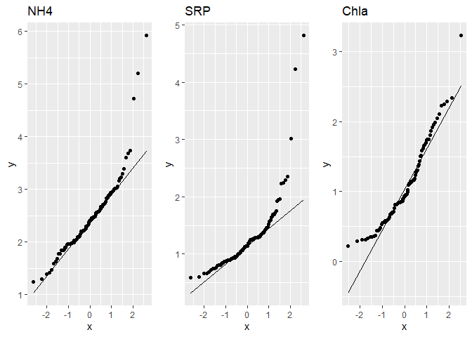
I would like to generate a plot over the specified columns of a data frame, use the column name as the title, and then arrange them using grid.arrange() from the package gridExtra.

Here is the code I currently have:

qq <- function(x){
  dlog %>%
  ggplot(aes(sample={{x}})) +
  stat_qq() +
  stat_qq_line() +
    labs(title=paste(x))
}

But I get an error with the labs() line.

After I've solved the title problem, how then can I arrange them all in a single window using grid.arrange()?

Here is a subset of my data. The columns I want to iterate this over are NH4, SRP and Chla.

dlog <- structure(list(Site = c("EAS5", "EAS5", "EAS17", "EAS17", "EAS38", 
"EAS38", "EMP5", "EMP5", "EMP17", "EMP17", "EMP38", "EMP38", 
"GTB5", "GTB5", "GTB17", "GTB17", "GTB38", "GTB38", "MNQ5", "MNQ5", 
"MNQ17", "MNQ17", "MNQ38", "MNQ38", "ROW5", "ROW5", "ROW17", 
"ROW17", "ROW38", "ROW38", "STU5", "STU5", "STU17", "STU17", 
"STU38", "STU38", "STJ8", "STJ8", "STJ17", "STJ17", "STJ30", 
"STJ30", "MIC8", "MIC8", "MIC17", "MIC17", "N3", "N3", "WAU8", 
"WAU8", "EG12", "EG12", "B5", "B5", "RAC8", "RAC8", "Q30", "Q30", 
"C6", "C6", "PWA8", "PWA8", "PWA17", "PWA17", "PWA30", "PWA30", 
"L260", "L260", "9561", "9561", "STO30", "STO30", "SHB8", "SHB8", 
"SHB17", "SHB17", "SHB30", "SHB30", "Man8", "Man8", "Man17", 
"Man17", "9574", "9574", "LVD8", "LVD8", "LVD17", "LVD17", "9570", 
"9570", "STJ5", "STJ5", "STJ17", "STJ17", "STJ38", "STJ38", "MIC5", 
"MIC5", "MIC17", "MIC17", "MIC38", "MIC38", "WAU5", "WAU5", "WAU17", 
"WAU17", "WAU38", "WAU38", "RAC5", "RAC5", "RAC17", "RAC17", 
"RAC38", "RAC38", "GH5", "GH5", "GH17", "GH17", "GH38", "GH38", 
"PWA5", "PWA5", "PWA17", "PWA17", "PWA38", "PWA38", "SHB5", "SHB5", 
"SHB17", "SHB17", "SHB38", "SHB38", "MAN5", "MAN5", "MAN17", 
"MAN17", "MAN38", "MAN38", "LUD5", "LUD5", "LUD17", "LUD17", 
"LUD38", "LUD38"), Ship = c("LE2", "LE2", "LE2", "LE2", "LE2", 
"LE2", "LE2", "LE2", "LE2", "LE2", "LE2", "LE2", "LE2", "LE2", 
"LE2", "LE2", "LE2", "LE2", "LE2", "LE2", "LE2", "LE2", "LE2", 
"LE2", "LE2", "LE2", "LE2", "LE2", "LE2", "LE2", "LE2", "LE2", 
"LE2", "LE2", "LE2", "LE2", "Guardian", "Guardian", "Guardian", 
"Guardian", "Guardian", "Guardian", "Guardian", "Guardian", "Guardian", 
"Guardian", "Guardian", "Guardian", "Guardian", "Guardian", "Guardian", 
"Guardian", "Guardian", "Guardian", "Guardian", "Guardian", "Guardian", 
"Guardian", "Guardian", "Guardian", "Guardian", "Guardian", "Guardian", 
"Guardian", "Guardian", "Guardian", "Guardian", "Guardian", "Guardian", 
"Guardian", "Guardian", "Guardian", "Guardian", "Guardian", "Guardian", 
"Guardian", "Guardian", "Guardian", "Guardian", "Guardian", "Guardian", 
"Guardian", "Guardian", "Guardian", "Guardian", "Guardian", "Guardian", 
"Guardian", "Guardian", "Guardian", "USGS", "USGS", "USGS", "USGS", 
"USGS", "USGS", "USGS", "USGS", "USGS", "USGS", "USGS", "USGS", 
"USGS", "USGS", "USGS", "USGS", "USGS", "USGS", "USGS", "USGS", 
"USGS", "USGS", "USGS", "USGS", "USGS", "USGS", "USGS", "USGS", 
"USGS", "USGS", "USGS", "USGS", "USGS", "USGS", "USGS", "USGS", 
"USGS", "USGS", "USGS", "USGS", "USGS", "USGS", "USGS", "USGS", 
"USGS", "USGS", "USGS", "USGS", "USGS", "USGS", "USGS", "USGS", 
"USGS", "USGS"), NH4 = c(2.98061863574394, 2.66722820658195, 
1.78002421300963, 2.31253542384721, 2.23108909128898, 1.89761985992753, 
1.89911798754855, 1.85159946958407, 2.45958884180371, 2.89591193827178, 
2.484906649788, 1.94304891677428, 2.76000994003292, 2.2512917986065, 
1.99333884262642, 2.14826773260969, 3.38777436133001, 3.02529107579554, 
2.66722820658195, 2.46809953147162, 1.30019166206648, 2.70136121295141, 
2.02551319965428, 2.89591193827178, 3.23474917402449, 2.82731362192903, 
2.45958884180371, 2.9391619220656, 2.39789527279837, 2.29455292129678, 
2.9338568698359, 3.60277675506052, 2.47653840011748, 2.51769647261099, 
2.2181159363676, 2.63188884013665, 2.17361471169709, 2.85186190313429, 
2.09433015417359, 2.88312332917134, 2.2213750375685, 2.2082744135228, 
2.2082744135228, 2.42568729012803, 2.46809953147162, 3.05635689537043, 
2.05540496385159, 2.32238772029023, 2.2213750375685, 2.57184857992181, 
1.67896397508271, 2.99972429482353, 2.43097830776244, 2.42036812865043, 
2.10169215061466, 2.56648663678042, 2.34660197841082, 2.94968833505258, 
1.83736998048011, 3.00864849882054, 1.63119940421561, 3.01798288248881, 
1.9643112344262, 2.59001713419062, 1.83736998048011, 1.9643112344262, 
2.20165917440409, 2.10169215061466, 1.41585316336144, 2.54788144894939, 
1.83736998048011, 1.9823798288367, 1.4655675420144, 2.7033726115511, 
1.24703229378638, 2.31055326264322, 1.38879124131848, 2.4518667957098, 
2.03208784529637, 1.9823798288367, 1.77833644889591, 2.57261223020711, 
1.58514521986506, 1.9643112344262, 1.98100146886658, 2.60859812213055, 
2.12106321637066, 2.29253475714054, 1.95727390770563, 2.02287119019144, 
2.39789527279837, NA, 1.98100146886658, NA, 5.91620206260743, 
NA, 2.71469474382088, NA, 2.23323501485925, NA, 2.67414864942653, 
NA, 2.82731362192903, NA, 2.04769284336526, NA, 2.47653840011748, 
NA, 5.2040066870768, NA, 2.56494935746154, NA, 2.55722731136763, 
NA, 2.72129542785223, NA, 2.09556092355972, NA, 3.15700042115011, 
NA, 4.72738781871234, NA, 3.73289633953071, NA, 2.37954613413017, 
NA, 2.73436750941958, NA, 2.58021682959233, NA, 3.68637632389582, 
NA, 3.19867311755068, NA, 2.24283508858827, NA, 1.96150224381515, 
NA, 2.83907846350861, NA, 2.1150499691472, NA, 3.29583686600433, 
NA), SRP = c(1.25561603747777, 1.2947271675944, 1.1999647829284, 
1.36609165380237, 1.24990173621434, 1.26976054486394, 1.15057202759882, 
1.1999647829284, 1.34547236659964, 1.25846098961001, 1.25561603747777, 
1.28923264827676, 1.27815220250019, 1.09192330051731, 1.13462272619114, 
1.32175583998232, 1.33762918913861, 1.42310833424261, 1.10525683138678, 
1.26412672714568, 1.11185751541813, 1.2947271675944, 1.13462272619114, 
1.31103187661934, 1.43508452528932, 1.18478998490916, 1.25561603747777, 
1.28647402583768, 1.29198368164865, 1.28923264827676, 1.28093384546206, 
1.2947271675944, 1.22377543162212, 1.28647402583768, 1.26129787094521, 
1.24126858906963, 0.8754687373539, 0.746687947487975, 0.916290731874155, 
1.07158361628019, 0.920282753143692, 0.936093359170335, 0.810930216216329, 
0.841567185678219, 0.951657875711446, 1.0681530811834, 0.751416088683921, 
0.936093359170335, 0.883767540168595, 0.955511445027436, 0.928219302739429, 
1.05082162483176, 1.01523067972906, 1.00795792039998, 0.76080582903376, 
0.8754687373539, 0.810930216216329, 0.845868267577609, 0.924258901523332, 
1.03318448334565, 0.8754687373539, 0.993251773010283, 0.966983846189673, 
1.06125650212434, 0.966983846189673, 1.00430160919687, 1.1314021114911, 
1.08856195281461, 0.900161349944271, 1.01160091167848, 0.896088024556636, 
0.896088024556636, 0.802001585472027, 0.900161349944271, 0.959350221334602, 
0.928219302739429, 1.46325540225602, 1.04027671165515, 0.904218150639886, 
0.887891257352457, 0.683096844706444, 0.657520002916794, 0.593326845277734, 
0.815364813284194, 0.662687973075237, 1.14422279992016, 0.828551817566148, 
1.12492959698548, 0.598836501088704, 0.72270598280149, 4.22537282462851, 
NA, 1.59736533119983, NA, 4.81218435537242, NA, 1.28370777234479, 
NA, 2.35137525716348, NA, 1.69744878975681, NA, 2.24389609664537, 
NA, 1.7509374747078, NA, 1.94591014905531, NA, 3.01062088604774, 
NA, 1.57484646766448, NA, 1.6467336971778, NA, 1.68639895357023, 
NA, 1.36863942588117, NA, 1.47017584510059, NA, 2.23001440015921, 
NA, 2.29152414563462, NA, 1.52388002407245, NA, 1.95586047990848, 
NA, 1.37624402526639, NA, 1.39128190263093, NA, 1.65632149833295, 
NA, 1.14103300455206, NA, 1.45861502269952, NA, 1.71199450075919, 
NA, 1.4036429994545, NA, 1.9213246735827, NA), Chla = c(0.63, 
0.84, 0.81, 2.34, 1.09, 3.23, 0.76, 0.85, 0.86, 0.84, 0.7, 2.11, 
0.56, 0.71, 0.56, 1.31, 0.61, 1.67, 0.81, 0.7, 0.96, 1.37, 1.24, 
1.75, 0.59, 0.89, 1.15, 1.52, 0.93, 2.29, 1.51, 0.6, 0.95, 2.05, 
0.9, 1.15, NA, NA, NA, NA, NA, NA, NA, NA, NA, NA, NA, NA, NA, 
NA, NA, NA, NA, NA, NA, NA, NA, NA, NA, NA, NA, NA, NA, NA, NA, 
NA, NA, NA, NA, NA, NA, NA, NA, NA, NA, NA, NA, NA, NA, NA, NA, 
NA, NA, NA, NA, NA, NA, NA, NA, NA, 0.93, 1.75, 1.19, 1.11, 0.33, 
1.99, 0.67, 1.59, 0.31, 0.58, 0.35, 2.25, 0.68, 0.85, 0.53, 1.16, 
0.22, 1.17, 1.02, 1.11, 0.46, 0.82, 0.31, 1.12, 2.23, 1.7, 0.68, 
1.28, 0.55, 1.74, 0.58, 0.99, 0.36, 1.17, 0.44, 1.44, 1.87, 0.95, 
0.35, 1.92, 0.44, 1.81, 0.81, 0.86, 0.83, 1.39, 0.48, 1.96, 0.84, 
1.62, 0.37, 1.3, 0.29, 1.66)), row.names = c(1L, 2L, 3L, 4L, 
5L, 6L, 7L, 8L, 9L, 10L, 11L, 12L, 13L, 14L, 15L, 16L, 17L, 18L, 
19L, 20L, 21L, 22L, 23L, 24L, 25L, 26L, 27L, 28L, 29L, 30L, 31L, 
32L, 33L, 34L, 35L, 36L, 38L, 39L, 40L, 41L, 42L, 43L, 44L, 45L, 
46L, 47L, 48L, 49L, 50L, 51L, 52L, 53L, 54L, 55L, 56L, 57L, 58L, 
59L, 60L, 61L, 62L, 63L, 64L, 65L, 66L, 67L, 68L, 69L, 70L, 71L, 
72L, 73L, 74L, 75L, 76L, 77L, 78L, 79L, 80L, 81L, 82L, 83L, 84L, 
85L, 86L, 87L, 88L, 89L, 90L, 91L, 93L, 94L, 95L, 96L, 97L, 98L, 
99L, 100L, 101L, 102L, 103L, 104L, 105L, 106L, 107L, 108L, 109L, 
110L, 111L, 112L, 113L, 114L, 115L, 116L, 117L, 118L, 119L, 120L, 
121L, 122L, 123L, 124L, 125L, 126L, 127L, 128L, 129L, 130L, 131L, 
132L, 133L, 134L, 135L, 136L, 137L, 138L, 139L, 140L, 141L, 142L, 
143L, 144L, 145L, 146L), class = "data.frame")

Thanks so much for your help!

scottyd22 · December 6, 2022, 2:37am

Below is one way to iterate over a list of column names and combine the plots in one layout. The function generates the plot for one column, sets the title of the plot to the column name, and then assigns the plot to the global environment as an object with the column name. Next, walk() is used to generate each plot by stepping through the target columns. Finally, the plots are combined into a single output using grid.arrange().

# columns to iterate over
target_cols = c('NH4', 'SRP', 'Chla')

qq <- function(x){
  p = ggplot(dlog, aes(sample=dlog[,x])) +
    stat_qq() +
    stat_qq_line() +
    labs(title=paste(x))

  assign(x, p, envir = globalenv())  
}

walk(target_cols, qq)

grid.arrange(NH4, SRP, Chla, ncol = 3)

nirgrahamuk · December 6, 2022, 9:46am

its also possible to do without walking the plots to global and manually gathering the results

target_cols = c('NH4', 'SRP', 'Chla')

qq <- function(x){
  p = ggplot(dlog, aes(sample=dlog[,x])) +
    stat_qq() +
    stat_qq_line() +
    labs(title=x)
}

grid.arrange(grobs=map(target_cols, qq),
             ncol = 3)

system · December 13, 2022, 9:47am

This topic was automatically closed 7 days after the last reply. New replies are no longer allowed.

If you have a query related to it or one of the replies, start a new topic and refer back with a link.