Hi,
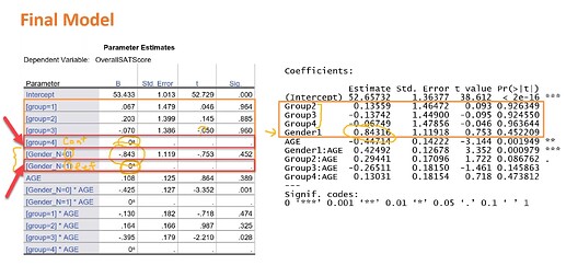
here below there is a comparison between regression table from SPSS and R.
In SPSS it gives us reference levels just placing 0 and dots in that table, on the other hand R is hiding/omitting refrence levels at all.
Is it possible to have in R an output like in SPSS ?
In SPSS the highest coded level is the reference level, contrary to R.
It would be good to have a possibility in R to set this in a custom way.
Is it possible to do it, to have it in R output ?
(Picture from K.Grace-Martin blog)
Reportedly expss should do this but I've never used it.
I imagine several of the major R tables packages will do the same. You might want to take a look at gt , flextable , kableExtra or gtsummary among others.
Sorry but this won't really be an answer to your question. My point is: why do you want to produce that misleading SPSS table at all? (unless your boss forces you to do so, of course). The group = 4, gender = 1 and group = 4 * AGE simply have no coefficients in the model, and I only find it misleading to put zeroesfor them in the table (a coefficient = 0 has a meaning, which is different). The right place to put your reference categories is the table caption, not the table itself.
There's another difference between the way SPSS and R include factors in their regressions. By default R takes the first level of a factor as reference category, which in your case is group = 1, gender = 0. This is not better per se than taking the last one, which apparently is what SPSS does, but increases the difficulty in comparing the two results. I suggest to manually define the reference category in R using relevel() if you want to have a comparable output.
This is not misleading, SPSS is just different, R conceals reference levels, but SPSS shows them with it's way.
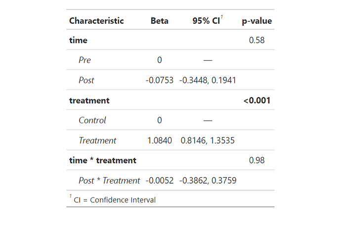
In SPSS I can now change level of the factor to the first level ( I found it finally in options). I do not want to use relevel, I want to show in R table a reference level like SPSS does. Partially I got it by means of using sjPlot package.
I have tried so far:
library(gtsummary)
library(sjPlot)

set.seed(1000)
my_data <- rbind(
  data.frame(time = "Pre", treatment = "Control", response = rnorm(100, mean=1)),
  data.frame(time = "Pre", treatment = "Treatment", response = rnorm(100, mean=2)),
  data.frame(time = "Post", treatment = "Control", response = rnorm(100, mean=1)),
  data.frame(time = "Post", treatment = "Treatment", response = rnorm(100, mean=2))
) %>% mutate(time = factor(time, levels = c("Pre", "Post"))) %>%
mutate(treatment = factor(treatment, levels = c("Control", "Treatment")))

model3 <- lm(response ~ time * treatment, data = my_data)


gtsummary::tbl_regression(model3,
  pvalue_fun = ~ style_pvalue(.x, digits = 2),
  estimate_fun = ~ style_number(.x, digits = 4)
) %>%
  add_global_p() %>%
  bold_p(t = 0.10) %>%
  bold_labels() %>%
  italicize_levels()


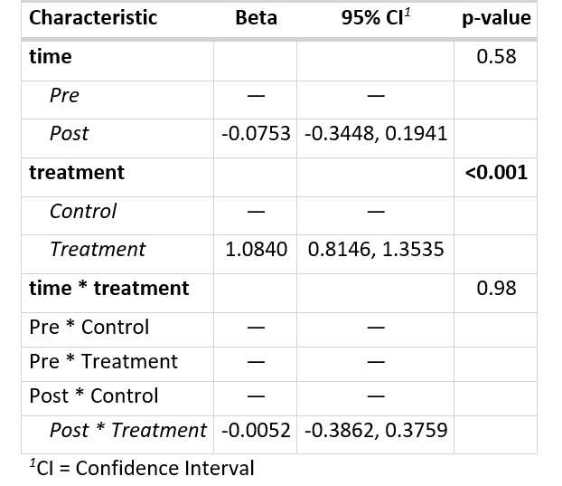
sjPlot::tab_model(model3, show.reflvl = TRUE)
My desired output is this:
Any help much appreciated, thank you.
I discovered that the discrepancy stemmed from the default handling of reference levels in categorical variables. Unlike the other page eg J.co beverages, which automatically set the highest coded level as the reference level, RStudio's behavior differed due to its reliance on the underlying R programming language. I learned that I could customize the reference levels in R by using the relevel() function to reorder factor levels.
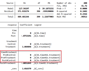
I have found it relatively easy to do it in Stata:
All base levels included, all base levels clearly visible.
Still trying to achieve the same in R.
Any help much appreciated.
You can hack gtsummary, to place 0 instead of —
like so :
library(gtsummary)
library(glue)

set.seed(1000)
my_data <- rbind(
  data.frame(time = "Pre", treatment = "Control", response = rnorm(100, mean=1)),
  data.frame(time = "Pre", treatment = "Treatment", response = rnorm(100, mean=2)),
  data.frame(time = "Post", treatment = "Control", response = rnorm(100, mean=1)),
  data.frame(time = "Post", treatment = "Treatment", response = rnorm(100, mean=2))
) %>% mutate(time = factor(time, levels = c("Pre", "Post"))) %>%
  mutate(treatment = factor(treatment, levels = c("Control", "Treatment")))

model3 <- lm(response ~ time * treatment, data = my_data)

newcode <- function (x, exponentiate, tidy_columns_to_report, estimate_fun,
                     pvalue_fun, conf.level)
{

  x <- modify_table_styling(x, columns = any_of("label"),
                            label = paste0("**", gtsummary:::translate_text("Characteristic"),
                                           "**"), hide = FALSE)
  estimate_column_labels <- gtsummary:::.estimate_column_labels(x)
  x <- modify_table_styling(x, columns = any_of("estimate"),
                            label = glue("**{estimate_column_labels$label}**") %>%
                              as.character(), hide = !"estimate" %in% tidy_columns_to_report,
                            footnote_abbrev = glue("{estimate_column_labels$footnote}") %>%
                              as.character(), fmt_fun = estimate_fun) %>% modify_table_styling(columns = any_of("estimate"),
                                                                                               rows = .data$reference_row == TRUE, missing_symbol = gtsummary:::get_theme_element("tbl_regression-str:ref_row_text",
                                                                                                                                                                      default = "0"))
  x <- modify_table_styling(x, columns = any_of("N"), label = glue("**{gtsummary:::translate_text('N')}**") %>%
                              as.character(), fmt_fun = style_number) %>% modify_table_styling(columns = any_of(c("N_obs",
                                                                                                                  "N_event", "n_obs", "n_event")), fmt_fun = style_number)
  x <- modify_table_styling(x, columns = any_of("ci"), label = glue("**{style_percent(conf.level, symbol = TRUE)} {gtsummary:::translate_text('CI')}**") %>%
                              as.character(), hide = !all(c("conf.low", "conf.high") %in%
                                                            tidy_columns_to_report), footnote_abbrev = ifelse(inherits(x$model_obj,
                                                                                                                       c("stanreg", "stanfit", "brmsfit", "rjags")), gtsummary:::translate_text("CI = Credible Interval"),
                                                                                                              gtsummary:::translate_text("CI = Confidence Interval"))) %>% modify_table_styling(columns = any_of("ci"),
                                                                                                                                                                                    rows = .data$reference_row == TRUE, missing_symbol = gtsummary:::get_theme_element("tbl_regression-str:ref_row_text",
                                                                                                                                                                                                                                                           default = "—"))
  x <- modify_table_styling(x, columns = any_of(c("conf.low",
                                                  "conf.high")), fmt_fun = estimate_fun)
  x <- modify_table_styling(x, columns = any_of("p.value"),
                            label = paste0("**", gtsummary:::translate_text("p-value"), "**"),
                            fmt_fun = pvalue_fun, hide = !"p.value" %in% tidy_columns_to_report)
  x <- modify_table_styling(x, columns = any_of("std.error"),
                            label = paste0("**", gtsummary:::translate_text("SE"), "**"), footnote_abbrev = gtsummary:::translate_text("SE = Standard Error"),
                            fmt_fun = function(x) style_sigfig(x, digits = 3), hide = !"std.error" %in%
                              tidy_columns_to_report) %>% modify_table_styling(columns = any_of("std.error"),
                                                                               rows = .data$reference_row == TRUE, missing_symbol = gtsummary:::get_theme_element("tbl_regression-str:ref_row_text",
                                                                                                                                                      default = "—"))
  x <- modify_table_styling(x, columns = any_of("statistic"),
                            label = paste0("**", gtsummary:::translate_text("Statistic"), "**"),
                            fmt_fun = function(x) style_sigfig(x, digits = 3), hide = !"statistic" %in%
                              tidy_columns_to_report) %>% modify_table_styling(columns = any_of("statistic"),
                                                                               rows = .data$reference_row == TRUE, missing_symbol = gtsummary:::get_theme_element("tbl_regression-str:ref_row_text",
                                                                                                                                                      default = "—"))
  x <- modify_table_styling(x, columns = c(where(is.numeric),
                                           -any_of(c("estimate", "conf.low", "conf.high", "p.value",
                                                     "std.error", "statistic", "N", "N_obs", "N_event",
                                                     "n_obs", "n_event"))), fmt_fun = function(x) style_sigfig(x,
                                                                                                               digits = 3))
  x
}

  assignInNamespace(".tbl_regression_default_table_header",
                    value = newcode,
                    ns = "gtsummary")
gtsummary::tbl_regression(model3,
                          pvalue_fun = ~ style_pvalue(.x, digits = 2),
                          estimate_fun = ~ style_number(.x, digits = 4)
) %>%
  add_global_p() %>%
  bold_p(t = 0.10) %>%
  bold_labels() %>%
  italicize_levels()
You could raise an issue Issues · ddsjoberg/gtsummary · GitHub asking to make the default missing place holder for estimates adjustable by a parameter away from the default emdash.
Hi and thank you NIr, very much for your effort but this is not really what I want.
I want to add three "empty reference" levels for interaction between time and treatment please.
Or generally speaking for two categorical variables.
Usually we reference a singular reference level, but here (when interaction occurs) there are actually 3: Pre * Control, Pre * Treatment, and Post * Control.
And for the sake of understanding and visibility I want to add this to tbl_regression output table.
Allegedly this woud be possible with the usage of gtsummary::modify_table_body() function but in spite of many trials and errors I was not able to achieve it. So I would be grateful if you could advise/show how to modify your code to to get it done.
I managed to get it in Stata.
Hi Nir Sir,
Could you please elaborate a bit what is happening in your code ?
This looks very advanced to me but I will go line-by-line through that.
Thank you very much in advance.
I understand that the concept is to modify gtsummary's hidden functions and adapt it to our needs, is it not ?
This is simply the code of gtsummary subfunction gtsummary:::.tbl_regression_default_table_header which handles some of the styling; I changed only the default symbol used for padding missing elements for estimate from - to 0 .
Ok thank you for kind explanation.
How to modify gtsummary::modify_table_body() to add those three reference levels I mentioned above ?
This topic was automatically closed 42 days after the last reply. New replies are no longer allowed.
If you have a query related to it or one of the replies, start a new topic and refer back with a link.


