Introducing new features in RavenR - R Views Submission

[rchlumsk]

Category: Homemade Package Vignette
Repo: GitHub - rchlumsk/RViews_RavenR_NewFeatures_Sept2021: Markdown file with reproducible examples corresponding to RViews post, discussing new features in RavenR.

---

Introducing new features in RavenR

RavenR is built to support the usage of the hydrologic modelling framework Raven, an open-source and supremely flexible software that allows the user to control all aspects of the model development and execution (i.e. model structure, discretization, outputs, etc.). Raven is used in both academia and practice for uses such as flood forecasting and operational reservoir management. The flexibility of Raven allows for a lot of great uses, but can be a little bit daunting for new users to pick up and visualize what is happening. RavenR can be helpful in this respect for new users, and also for more experienced users to help them save some time in their file preparations and analyses.

The introductory vignette (browseVignettes("RavenR")) provides a more comprehensive review of the RavenR basics, so we will leave that alone for now, and instead jump into some new and interesting features of RavenR. These will be available in the next release to CRAN, and are already available in the developmental Github version of the package.

Load the RavenR library

The RavenR library can be installed from CRAN or from Github with the devtools package. For these new features, we will be working with the developmental Github version.

library(devtools)
devtools::install_github("rchlumsk/RavenR")

Update: v2.1.4 of RavenR with the features discussed in this article is now live on CRAN and can be installed directly with:

install.packages("RavenR")

We can load the RavenR package, and some additional packages we will need while we are here.

library(RavenR)
library(ggplot2)
library(DiagrammeR)
library(dplyr)
library(weathercan)

library(knitr)
library(kableExtra)

Downloading and running Raven

A nice utility in the new version of RavenR are functions to directly download and run Raven, saving the hassle of managing and moving around a Raven executable, which can cause issues particularly for new users. Instead, the executable is downloaded for the user's system and placed within the installed RavenR package's extdata/ folder (found with system.file). This works well in Windows, although compilation may be required for non-Windows users. The executable may be automatically (or manually) placed in the RavenR/extdata folder for use with rvn_run.

rvn_download()

# check if Raven.exe is found in RavenR/extdata
rvn_download(check=TRUE)

## [1] "Raven.exe found in C:/opt/R/R-current/R-4.1.1/library/RavenR/extdata"

## [1] TRUE

We can now run the Raven executable without having the locate, copy, or link to the desired executable. To test this functionality, the snippet below will download the Raven Tutorial files, and run the Irondequoit model (see console output with showoutput=TRUE).

url<-"http://raven.uwaterloo.ca/files/RavenTutorialFiles.zip"
destfile<-paste(getwd(),"/RavenTutorialFiles.zip",sep="")
download.file(url,destfile)
destdir<-paste(getwd(),"/RavenTutorialFiles",sep="")
dir.create(destdir)
unzip(zipfile=destfile,exdir=destdir)
file.remove(destfile)

# Irondequoit example
rvn_run(indir="./RavenTutorialFiles/Irond",
        outdir="./RavenTutorialFiles/Irond/output/",
         showoutput=FALSE)

# show produced output files
list.files("./RavenTutorialFiles/Irond/output/")

## [1] "Raven_errors.txt"          "run1_Hydrographs.csv"     
## [3] "run1_solution.rvc"         "run1_WatershedStorage.csv"

You may supply the model prefix to the rvi file to rvn_run, although in this case it was able to detect it automatically as the only *.rvi file in the provided directory.

Starting with a model structure and parameter set

The model structure defines all of the connections in the model - which water storage units are in the model, and how they are connected. Building this initial model structure is a necessary task to begin any modelling, but can be daunting for new users who are not yet comfortable with this. Luckily, a very simple script that houses the template files from the Raven User's Manual will write the model template of your choice to file to get you started. These templates include many commonly used models in the literature (such as GR4J and HMETS).

# write the HBV-EC template to file
rvn_rvi_write_template(modelname="HBV-EC", 
                       filename='HBV-EC_template.rvi',
                       author='Robert Chlumsky')

The template function includes the command CreateRVPTemplate in the *.rvi file, which will tell Raven to generate a template of the rvp file with all of the necessary parameters and formatting. In a typical model-building process, this would be one of the next steps. Here, we can use the rvn_run function directly within R to run Raven and generate this template file, and view the :SoilParameterList section of the rvp file.

rvn_run(fileprefix="HBV-EC_template")

# view :SoilParameterList table
dt <- read.table("HBV-EC_template.rvp_temp.rvp", 
           skip=65, nrows=6, fill=TRUE)
colnames(dt) <- lapply(dt[1,],FUN=function(x) ifelse(rvn_substrLeft(x,1)==":",rvn_substrMLeft(x,1),x))
dt[-1,] %>%   
  kbl() %>% 
    kable_material(c("striped", "hover"))

	Parameters,	POROSITY,	HBV_BETA,	PET_CORRECTION,	FIELD_CAPACITY,	SAT_WILT,	MAX_CAP_RISE_RATE,	MAX_PERC_RATE,	BASEFLOW_COEFF,	BASEFLOW_N,
2	:Units,	-,	-,	-,	-,	-,	-,	-,	-,	-,
3	[DEFAULT],	**,	**,	**,	**,	**,	**,	**,	**,	**,
4	SOILCLASS1,	**,	**,	**,	**,	**,	**,	**,	**,	**,
5	SOILCLASS2,	**,	**,	**,	**,	**,	**,	**,	**,	**,
6	…

We can also quickly generate a table of initial parameter values and ranges for each required parameter with rvn_rvi_getparams, which is very useful for eventually configuring a calibration exercise.

rvn_rvi_read("HBV-EC_template.rvi") %>% 
  rvn_rvi_getparams() %>% 
  slice(c(1,2,16,17)) %>% # subset for presentation
    kbl() %>% 
      kable_material(c("striped", "hover"))

param	class_type	units	auto	default	min	max
FOREST_COVERAGE	LULT	[0..1]	False	0	0	1.0
LAKE_PET_CORR	LULT	[0..1]	False	1.0	0.0	2.0
BASEFLOW_N	SOIL	[-]	False	5	-9999	-9999.0
SNOW_SWI	GLOBAL	[0..1]	True	0.05	0.0	0.5

Examining the model structure

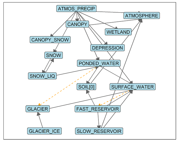
Visualizing the model structure network can get complicated, especially for some of the more advanced models with conditional connections. We can create these with either ggplot2 or DiagrammeR packages under the hood. Let's examine the structure of the template file we created using the ggplot2 version.

rvn_rvi_read("HBV-EC_template.rvi") %>% 
  rvn_rvi_connections() %>% 
  rvn_rvi_process_ggplot(., lbl_size=0.7, arrow_size = 0.3)

The labels are repelled from one another using the same core functionality as the ggrepel package. The connections between each storage unit in Raven is shown, with conditional connections shown as a dashed orange line.

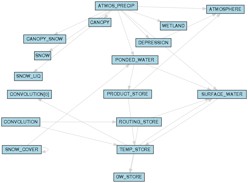
Let's contrast this model structure to the GR4J structure, which we will make with the DiagrammeR version of the function. The DiagrammeR::render_graph function is used to actually produce this plot. We will again use the rvi template function to first generate an rvi file to read, then map its structure.

rvn_rvi_write_template(modelname="GR4J", 
                       filename='GR4J_template.rvi')

rvn_rvi_read("GR4J_template.rvi") %>% 
  rvn_rvi_connections() %>% 
  rvn_rvi_process_diagrammer(., lbl_size=0.6) %>% 
  render_graph()

The GR4J structure is conceptually simpler, including no consideration of glacial processes. The key note here is that these plots are important to view as they tell you a lot about your model, and they can now be easily generated for any Raven rvi file.

Preparing meteorological input data

This may be the section with the best time-saving tools in all of RavenR. Preparing the input data for any model can often be the most time-consuming step in the whole process, and Raven requires meteorological data free of missing values (meteorological data can be considered a boundary condition for hydrologic models).

We begin by finding all stations with data between 2002 and 2006, and that exist within 50km of the Glen Allan station (as arbitrary parameters for our search).

# library(weathercan)
glen_stn <- weathercan::stations_search(name="Glen Allan", interval = "day")[1,]
all_stns <- weathercan::stations_search(coords=c(glen_stn$lat, glen_stn$lon), dist=50, 
              interval="day", starts_latest = 2002,
             ends_earliest = 2006)
all_stns$station_name

## [1] "GLEN ALLAN"                       "FERGUS MOE"                      
## [3] "FERGUS SHAND DAM"                 "MOUNT FOREST (AUT)"              
## [5] "REGION OF WATERLOO INT'L AIRPORT" "WROXETER"                        
## [7] "ROSEVILLE"                        "STRATFORD WWTP"

This search yields 8 stations within a 50km radius of our point of interest. We can now download the meteorological data for all 8 stations in one line with weathercan, which will store it all in a single tibble.

weather_data <- weather_dl(station_ids = all_stns$station_id, 
                           start = "2002-10-01", 
                           end = "2010-10-01",
                           interval="day")

Now, let's say we just want three particular meteorological stations to be included in our model: Glen Allan, Mount Forest, and Wroxeter. Why would we bother downloading all 8? Well, there may not be enough data in just the three stations to spatially interpolate all of the missing values - it's possible that there are simultaneous gaps in the data, especially with a longer time series and only three stations. To mitigate this risk and improve the data quality upon interpolation, we download all 8 stations and use all 8 to infill missing values in our favourite 3. Of course, this is optional, but this capability is built into the RavenR function rvn_met_interpolate.

So let's define our stations of interest, and perform the interpolation first with just the three stations of interest.

favourite_stations <- all_stns[c(1,4,6),]
favourite_stations$station_name

## [1] "GLEN ALLAN"         "MOUNT FOREST (AUT)" "WROXETER"

new_wd <- weather_data %>% 
  select(station_name, station_id, lat,lon,elev, date,
         max_temp, min_temp, total_precip) %>% 
  filter(station_name %in% favourite_stations$station_name) %>% 
 rvn_met_interpolate(weather_data=.)

## Warning in rvn_met_interpolate(weather_data = .): missing data for %s, more
## stations may be required: 2008-01-24

## Warning in rvn_met_interpolate(weather_data = .): missing data for %s, more
## stations may be required: 2008-01-24

## Warning in rvn_met_interpolate(weather_data = .): missing data for %s, more
## stations may be required: 2008-01-24

## Warning in rvn_met_interpolate(weather_data = .): rvn_met_interpolate: Some key
## columns still contain NA values, additional data or alternative interpolation
## may be required.

The warnings show that we have missing data in all three stations on 2008-01-24 that cannot be reconciled. When we run this with data from all 8 stations, we avoid this issue.

new_wd <- weather_data %>% 
  select(station_name, station_id, lat,lon,elev, date,
         max_temp, min_temp, total_precip) %>% 
 rvn_met_interpolate(weather_data = ., 
                              key_stn_ids = favourite_stations$station_id)

In either case, the resulting interpolated data frame has data pertaining only to our stations of interest. We can therefore pipe the data frame directly to the rvt writing function for meteorlogical data, rvn_rvt_write_met. This function will automatically parse out the stations, write appropriate file names, and parse out the metadata for each station (latitude/longitude, elevation) in the data frame into a separate rvt file, which we will need to supply to our model.

new_wd %>% 
  rvn_rvt_write_met()

## [1] "Imported data from 3 stations"

## rvn_rvt_write_met: Done writing to met_GLEN_ALLAN.rvt

## rvn_rvt_write_met: Done writing to met_MOUNT_FOREST_(AUT).rvt

## rvn_rvt_write_met: Done writing to met_WROXETER.rvt

## rvn_rvt_write_met: Done writing rvt files for 3 station(s)

## rvn_rvt_write_met: Done writing station data to met_stndata.rvt

## [1] TRUE

The data files are (by default) named with a 'met_' prefix for file organization, while the station metadata file would typically be found in your main *.rvt file, which would also point to the longer format time series data files with the :RedirectToFile command.

Conclusion

This article is intended to bring to light some of the new (and as hopefully demonstrated, very useful!) capabilities within the RavenR package. The hope is that the investment of time into developing these tools will allow others to save some time and headaches in working with their Raven models. Look for a new version of RavenR on CRAN soon with these new tools included, and if you have any thoughts to share about the RavenR package or this article, feel free to share them with me via email or on Github discussions.

Thank you!

A quick thank you a few R people: James Craig for his endless help in all things, and also to my other co-authors on the RavenR project, Sarah Grass, Simon Lin, Genevieve Brown, Leland Scantlebury, and Rezgar Arabzadeh. I also want to thank Kevin Shook and Paul Whitfield of the CSHS-hydRology project for giving me the R bug years ago.

---

This is a submission to the R Views Call for Documentation. For more information see rviews.rstudio.com.