I created two GAM models, one looking at the relationship between the daily precipitation depth (mm) and the daily increase in stream discharge (m3/s) before a disturbance (i.e. the control), and one looking at the relationship between the daily precipitation depth (mm) and the daily increase in stream discharge (m3/s) after a disturbance (i.e. the treatment), and want to see if there is a difference in the relationship pre-and post disturbance.
I began by uploading two csv files and creating two data objects (one for pre-disturbance and one for post-disturbance) using the code:
preOutlierRem.dat <- read.csv("PrecipDischargeOutliersRemPre.csv")
postOutlierRem.dat <- read.csv("PrecipDischargeOutliersRemPost.csv")
The format of the data for preOutlierRem.dat is shown below:
Date, Discharge, Precipitation, DailyChange, DailyIncrease
2010-05-01, 0.941, 2.8, 0.000, 0.000000000
2010-05-02, 0.528, 28.8,  -0.413, 0.000000000
2010-05-03, 0.422, 0.0,  -0.106, 0.000000000
2010-05-04, 0.366, 2.8, -0.056, 0.000000000
2010-05-05, 1.381, 12.0, 1.015, 1.015000000
2010-05-06, 0.836,  0.0, -0.545,  0.000000000
2010-05-07, 0.639,  0.0, -0.197,   0.000000000```
And the format of the data for postOutlierRem.dat is shown below
Date, Discharge, Precipitation, DailyChange, DailyIncrease
2010-05-01, 0.941, 2.8, 0.000, 0.000000000
2010-05-02, 0.528, 28.8, -0.413, 0.000000000
2010-05-03, 0.422, 0.0, -0.106, 0.000000000
2010-05-04, 0.366, 2.8, -0.056, 0.000000000
2010-05-05, 1.381, 12.0, 1.015, 1.015000000
2010-05-06, 0.836,  0.0,  -0.545, 0.000000000
2010-05-07, 0.639, 0.0, -0.197, 0.000000000
As shown above, I have two sets of time series data (one representing a pre-disturbance scenario, and the other representing a post-disturbance scenario). Each dataset contains data for the daily precipitation depth (mm), daily discharge (m3/s), daily change in stream discharge (m3/s), and daily increase in stream discharge (m3/s).
I want to model the relationship between daily precipitation depth (mm) and daily increase in stream discharge, both pre-and post disturbance and develop some sort of equation to represent the relationship between daily precipitation depth (mm) and daily increase in stream discharge.
I thought that a GAM model would be an appropriate method for modelling the relationship between daily precipitation depth and the daily increase in stream discharge. As such, I created two GAM models: one to represent the pre-disturbance scenario (named "preGAM"), and one to represent the post-disturbance scenario (named "postGAM"), as shown in the code below:
preGAM <- gam(preOutlierRem.dat$DailyIncrease ~ s(preOutlierRem.dat$Precipitation))
postGAM <- gam(postOutlierRem.dat$DailyIncrease ~ s(postOutlierRem.dat$Precipitation))```
I plotted each of the GAM models (preGAM and postGAM) using the code
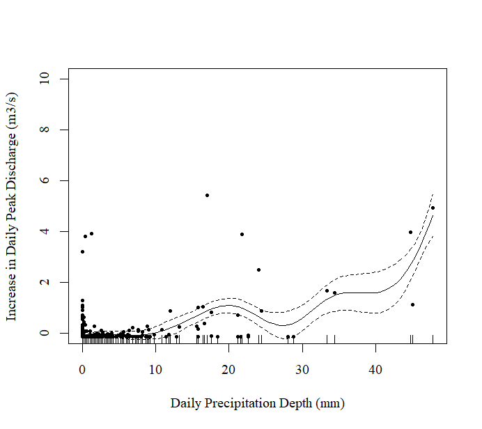
plot.gam(preGAM, residuals = TRUE, xlab = "Daily Precipitation Depth (mm)", ylab = "Increase in Daily Peak Discharge (m3/s)", family = "A", ylim = c(0,10), pch = 19, cex = .5)
plot.gam(postGAM, residuals = TRUE, xlab = "Daily Precipitation Depth (mm)", ylab = "Increase in Daily Peak Discharge (m3/s)", family = "A", ylim = c(0,10), pch = 19, cex = .5)
This code returned the following plot for the pre-disturbance scenario
and the following plot for the post-disturbance scenario
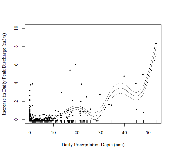
It can be observed in the above plots that there is some sort of increase in the effect of precipitation depth on the increase in stream discharge in the post-disturbance scenario (i.e., there is a much greater slope in the second plot compared to the first).
When I view the summary of the models for the pre-disturbance and post-disturbance GAM models, I receive the following output for the pre-development scenario:
> summary(preGAM) # r-squared = 0.355

Family: gaussian
Link function: identity

Formula:
preOutlierRem.dat$DailyIncrease ~ s(preOutlierRem.dat$Precipitation)

Parametric coefficients:
            Estimate Std. Error t value Pr(>|t|)
(Intercept)  0.12748    0.01849   6.894 1.52e-11 ***
---
Signif. codes:  0 ‘***’ 0.001 ‘**’ 0.01 ‘*’ 0.05 ‘.’ 0.1 ‘ ’ 1

Approximate significance of smooth terms:
                                     edf Ref.df     F p-value
s(preOutlierRem.dat$Precipitation) 8.511  8.931 34.16  <2e-16 ***
---
Signif. codes:  0 ‘***’ 0.001 ‘**’ 0.01 ‘*’ 0.05 ‘.’ 0.1 ‘ ’ 1

R-sq.(adj) =  0.355   Deviance explained = 36.5%
GCV = 0.1907  Scale est. = 0.18739   n = 548
I also receive the following output for the post-development scenario
summary(postGAMRem) # R-squared = 0.473

Family: gaussian
Link function: identity

Formula:
postGAMRem.dat$DailyIncrease ~ s(postGAMRem.dat$Precipitation)

Parametric coefficients:
            Estimate Std. Error t value Pr(>|t|)
(Intercept)   0.1306     0.0125   10.45   <2e-16 ***
---
Signif. codes:  0 ‘***’ 0.001 ‘**’ 0.01 ‘*’ 0.05 ‘.’ 0.1 ‘ ’ 1

Approximate significance of smooth terms:
                                  edf Ref.df     F p-value
s(postGAMRem.dat$Precipitation) 8.905  8.997 109.6  <2e-16 ***
---
Signif. codes:  0 ‘***’ 0.001 ‘**’ 0.01 ‘*’ 0.05 ‘.’ 0.1 ‘ ’ 1

R-sq.(adj) =  0.473   Deviance explained = 47.7%
GCV = 0.17269  Scale est. = 0.17113   n = 1096
Does anybody have any advice on how to proceed from this point determine the relationship between precipitation and the daily increase in stream discharge under both the pre-disturbance and post-disturbance scenarios?
TIA