Interpreting Residuals v Fitted

[sean1]

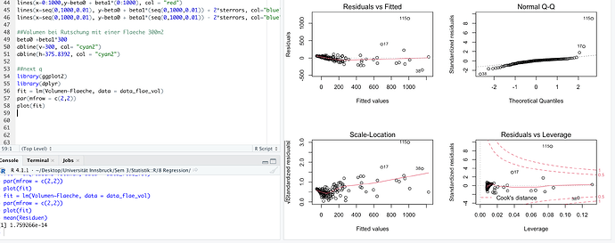
I hope the screenshot is visible. I am working with area (x) against volume (y) of a landslide. I am new to statistics, I am unsure if this is a good fit or not? As most residuals are close to 0? Thank you in advance!!

[FJCC]

Whether a fit is good is very dependent on the context. Ideally all of the plots except Normal Q-Q would show points randomly distributed with no slope or structure and the Normal Q-Q would be a perfect line. That is not exactly true for your data. The Residual vs Fitted has a pattern at low Fitted values where the Residuals are first positive then slowly move to negative values. The scatter of the residuals also increases from left to right. This suggests that the relationship between Volumen and Flaeche is somewhat different when Volumen is low and high. The Scale-Location plot shows similar patterns. And point 115 is obviously notable in every plot. Whether these deviations from the ideal are "bad" depends on the field of application. In a tightly controlled and well understood situation, e.g. the measured concentration of a solute in a carefully controlled solution, such deviations might be very bad. In many "real world" situation where the linear relationship is known or suspected to be only approximate, such deviations would probably be perfectly acceptable.
I have never considered landslides. Is there a strong reason to expect a very linear relationship? If not, nothing in those plots makes me think "wow, that's no linear!" But remember, I'm just a random guy on the internet.
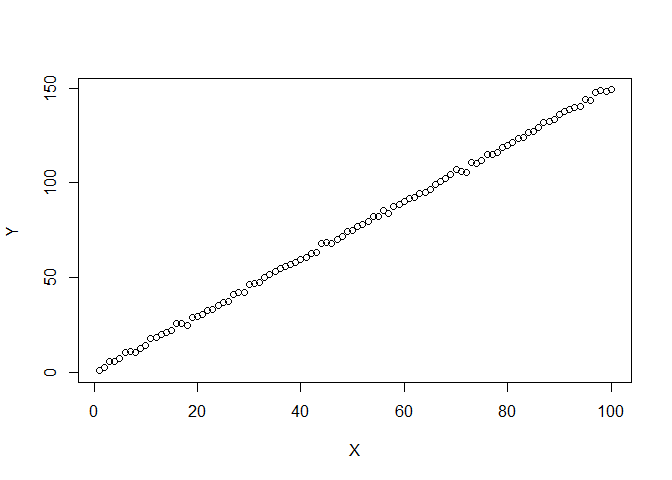
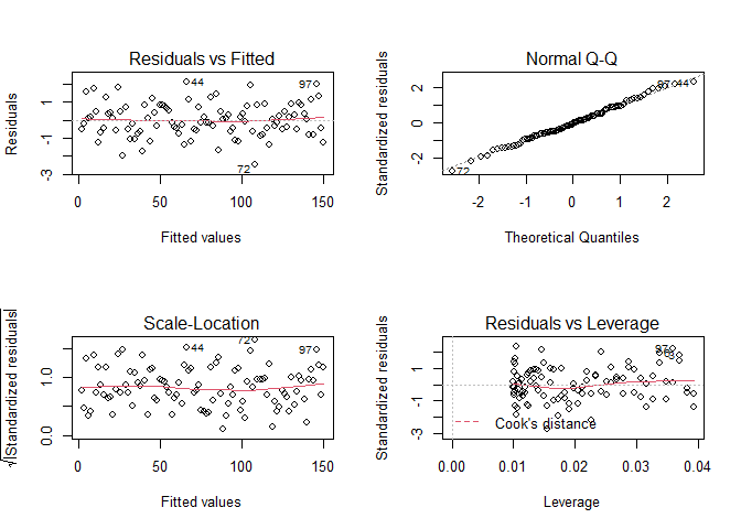
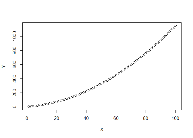
The examples below show one data set that is very close to linear and another that is definitely not linear. The second shows VERY obvious structure in the plots of the fit. The two examples might help you judge how non-ideal your plots are.

set.seed(123)
DF <- data.frame(X=1:100,Y=1:100*1.5+rnorm(100))
plot(DF)

FIT <- lm(Y~X,data = DF)
par(mfrow = c(2,2))
plot(FIT)

DF2 <- data.frame(X=1:100,Y=(1:100)^2*0.1+1:100*1.5+rnorm(100))  
par(mfrow=c(1,1))
plot(DF2)

FIT2 <- lm(Y~X,data = DF2)
par(mfrow = c(2,2))
plot(FIT2)

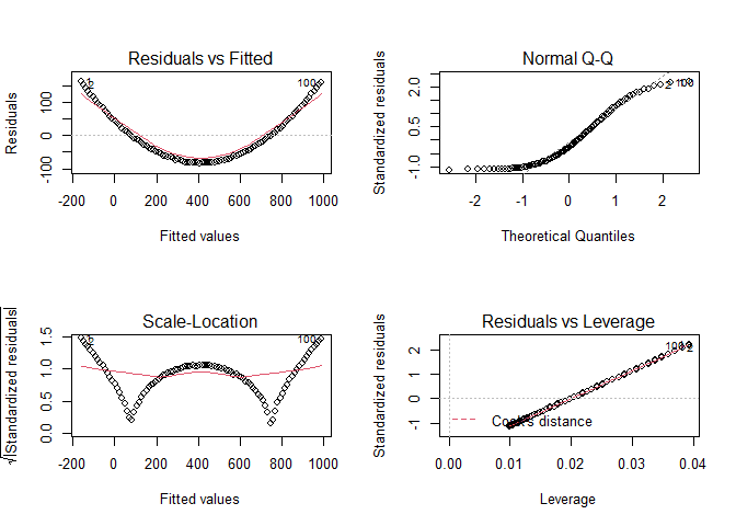
^{Created on 2021-12-21 by the reprex package (v2.0.1)}

[sean1]

Excellent, Thank you so much!!!!

[M_AcostaCH]

You could improve understand maybe if make Shapiro-Wilk test or Kolmogorov. Is easy and the interpretation like p-value < 0.05. This is for identifed normal distribution in the data:

x <- runif(100) 
x.test <- shapiro.test(x)
print(x.test)

# p-value = 4.082e-05

The data not have normal distribution.

When you make a regression model, it must meet the assumptions of normality, homoscedastic, so that the prediction makes sense.

[startz]

Normality is of very little importance for a regression, especially if there are a large number of observations.