There are 3 steps:
- decide on a model
- fit the model for each variable
- predict new values
Model
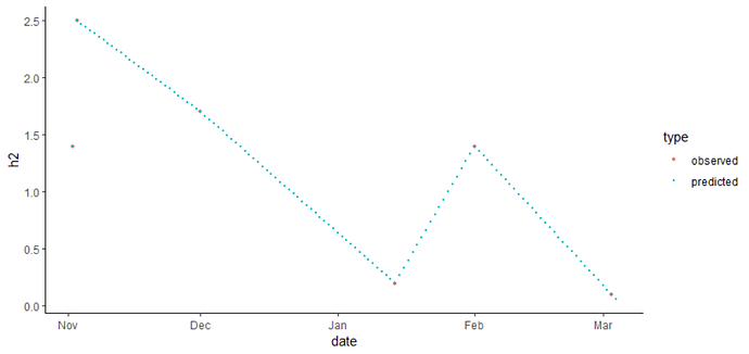
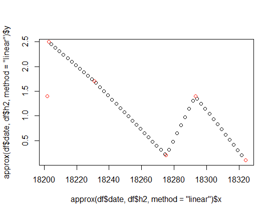
You mention linear, that would be done with the function lm(). A generic way to make a smooth interpolation is loess(). Many other models do exist.
Fitting
In a base R approach, you can do the fitting like this:
mod_h2 <- lm(h2 ~ date, data = df)
mod_n2 <- loess(n2 ~ as.numeric(date), data = df)
mod_co2 <- lm(log(co2) ~ date, data = df)
You can use summary() to get details, and of course you need to check the assumptions (e.g. distribution of the residuals).
Prediction
Each model type has an associated predict() function, which takes the model, and a set of new x values, and predict the corresponding y values according to the model.
Reprex
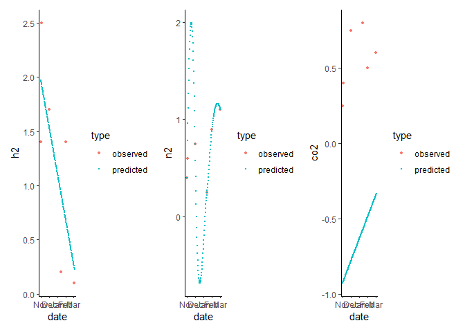
So a complete example with some bad models and clumsy plotting:
library(dplyr)
#>
#> Attaching package: 'dplyr'
#> The following objects are masked from 'package:stats':
#>
#> filter, lag
#> The following objects are masked from 'package:base':
#>
#> intersect, setdiff, setequal, union
library(tibble)
library(ggplot2)
library(lubridate)
#>
#> Attaching package: 'lubridate'
#> The following objects are masked from 'package:base':
#>
#> date, intersect, setdiff, union
df <- data.frame("date"=c("20191102", "20191103", "20191201", "20200114", "20200201",  "20200303"),
                   "h2" = c(1.4,   2.5,  1.7,  0.2,  1.4,  0.1),
                   "n2"=c(0.4, 0.6, 0.75, 0.25, 0.9, 1.1),
                   "co2"=c(0.25, 0.40, 0.75, 0.8,  0.5, 0.6)) %>%
  mutate(date=ymd(date))
mod_h2 <- lm(h2 ~ date, data = df)
mod_n2 <- loess(n2 ~ as.numeric(date), data = df)
mod_co2 <- lm(log(co2) ~ date, data = df)
new_df <- data.frame(date = seq(from = as.Date("2019-11-01"),
to = as.Date("2020-03-04"),
by="day"))
new_df <- new_df %>%
mutate(h2 = predict(mod_h2, newdata = new_df),
n2 = predict(mod_n2, newdata = new_df),
co2 = predict(mod_co2, newdata = new_df))
df_both <- add_column(df, type = "observed") %>%
bind_rows(add_column(new_df, type = "predicted"))
p_h2 <- ggplot(df_both) +
theme_classic() +
geom_point(aes(x = date, y = h2, color = type, size = type)) +
scale_size_discrete(range = c(1, .2))
#> Warning: Using size for a discrete variable is not advised.
p_n2 <- ggplot(df_both) +
theme_classic() +
geom_point(aes(x = date, y = n2, color = type, size = type)) +
scale_size_discrete(range = c(1, .2))
#> Warning: Using size for a discrete variable is not advised.
p_co2 <- ggplot(df_both) +
theme_classic() +
geom_point(aes(x = date, y = co2, color = type, size = type)) +
scale_size_discrete(range = c(1, .2))
#> Warning: Using size for a discrete variable is not advised.
patchwork::wrap_plots(p_h2, p_n2, p_co2)
#> Warning: Removed 2 rows containing missing values (geom_point).

Created on 2023-01-05 by the reprex package (v2.0.1)


