Here is the function I use to create the graph:
pets<-function(taxa, time, obs_type=NULL, fauna=NULL, plot=T, colours=c("red","darkgreen","blue","yellow","purple"),persistence="palegreen", absence="pink", end=NULL){
res<-NULL
if(is.null(obs_type)){
data<-as.data.frame(cbind(taxa,time,rep("observation",length(taxa))))
}else{
data<-as.data.frame(cbind(taxa,time,obs_type))
}
species<-unique(data[,1])
if(!(is.null(fauna))){
checksp<-species[-which(species %in% fauna)]
if (length(checksp)>0){
stop(paste("There are species absent in the checklist:",checksp))
}
}
res$observations<-length(which(!(is.na(time))))
res$NA_observation<-length(which(is.na(time)))
anni<-NULL
for(sp in 1:length(species)){
#sp<-1
anni[[sp]]<-as.numeric(unique(data[which(data[,1]==species[sp]),2]))
}
start<-min(unlist(anni),na.rm=T)
if(is.null(end)){
end<-max(unlist(anni),na.rm=T)
}
nasp<-rep(0,length(species))
for(sp in 1:length(species)){
#sp<-1
if(is.na(min(anni[[sp]]))){
nasp[sp]<-1
}
}
tipidati<-unique(data[,3])
tipidati<-as.character(tipidati[order(tipidati)])
last_sp<-rep(NA,length(species))
first_sp<-last_sp
for (c in 1:length(species)){
#c<-1
annisp<-anni[[c]][which(!is.na(anni[[c]]))]
if(length(annisp)>0){
last_sp[c]<-max(anni[[c]],na.rm=T)
first_sp[c]<-min(anni[[c]],na.rm=T)
}
}
last_sp2<-last_sp
last_sp2[which(is.na(last_sp))]<-min(last_sp,na.rm=T)-1
ordine<-order(last_sp2)
species2<-species[ordine]
last_sporder<-last_sp[ordine]
first_sporder<-first_sp[ordine]
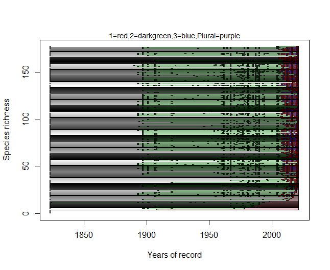
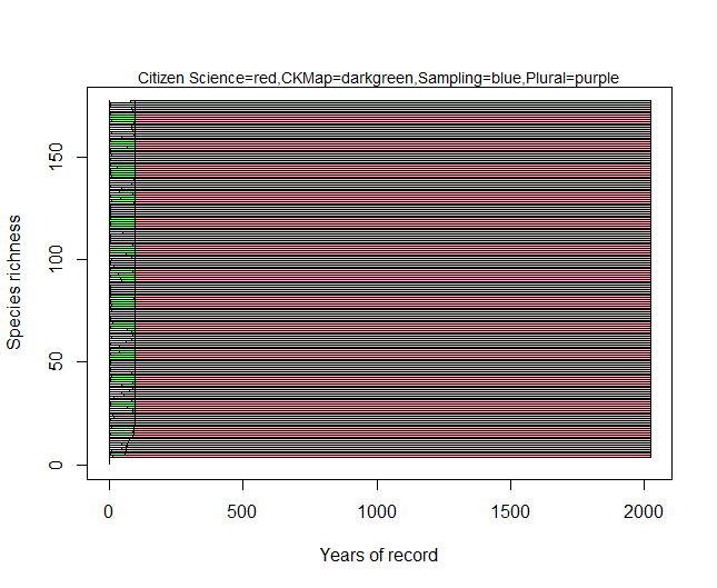
if(plot){
plot(rbind(c(start-2,0),c(end,length(species))),type="n",ylab="Species richness",xlab="Years of record")
mtext(paste(paste(c(tipidati,"Plural"),"=",col=c(colours[1:length(tipidati)],colours[length(colours)]),sep=""),collapse=","),cex=0.9)
#massimo per ogni specie
for (sp in 1:length(species2)){
#sp<-sp+1
datisp<-data[which(data[,1]==species2[sp]),]
annir<-datisp[!duplicated(cbind(datisp[,2],datisp[,3])),]
annisp<-as.numeric(unique(annir[,2]))
if(length(which(!(is.na(annisp))))>0){
mi<-min(annisp, na.rm=T)
ma<-max(annisp, na.rm=T)
rect((mi-1.5),(sp-0.5),(ma)-0.5,(sp+0.5),col=persistence,border=T)
rect((ma-1.5),(sp-0.5),(end)-0.5,(sp+0.5),col=absence,border=T)
}
for (quad in 1:length(annisp)){
#quad<-1
tipi1<-annir[which(annir[,2]==annisp[quad]),]
tipol<-tipi1[,3]
match<-which(tipidati %in% tipol)
if(length(match)>0){
if(length(match)==1){
colore<-colours[match]
}
if(length(match)>1){
colore<-colours[length(colours)]
}
rect(((annisp[quad])-1.5),(sp-0.5),((annisp[quad])-0.5),(sp+0.5),col=colore,border=T)
}
arrows((start-2.5),(sp-0.5),(annisp[quad]-0.5),(sp-0.5), length =0)
}
if(length(match)==0){
colore<-"grey"
rect((start-2.5),(sp-0.5),(start-1.5),(sp+0.5),col=colore,border=T)
}
}
}
res$extinctionP<-sum(end-last_sp, na.rm=T)/sum((end-first_sp+1), na.rm=T)
res$table<-as.data.frame(cbind(species2,first_sporder,last_sporder))
return(res)
}
I then only have to load my database and run the function:
vda <- read.csv("D:/...................Database_analysis.csv",sep=";",dec=",",header=TRUE)
str(vda)

'data.frame':	24909 obs. of  15 variables:
 $ SPECIE_EU      : Factor w/ 177 levels "Aglais_io","Aglais_urticae",..: 1 1 1 1 1 1 1 1 1 1 ...
 $ AUTORE_ANNO_EU : Factor w/ 75 levels "(Bergsträsser_1779)",..: 43 43 43 43 43 43 43 43 43 43 ...
 $ SPECIE_ITA     : Factor w/ 180 levels "Aglais_urticae_",..: 84 84 84 84 84 84 84 84 84 84 ...
 $ AUTORE_ANNO_ITA: Factor w/ 76 levels "(Bergsträsser_1779)",..: 47 47 47 47 47 47 47 47 47 47 ...
 $ REGIONE        : Factor w/ 1 level "Valle_d_Aosta": 1 1 1 1 1 1 1 1 1 1 ...
 $ LOCALITA_      : Factor w/ 283 levels "","(Saint-Rhémy-en-Bosses)",..: 64 221 59 59 234 39 59 74 89 94 ...
 $ STAZIONE       : Factor w/ 449 levels "","\"alcune_localita_della_media_valle_di_Champorcher\"",..: 1 1 1 1 95 1 1 1 1 1 ...
 $ FONTE          : Factor w/ 14620 levels "A._Casale_(Com._Verb.)",..: 14605 14605 14545 25 14524 14524 14524 14524 14524 14524 ...
 $ ANNO           : int  1898 1898 1963 1965 1968 1968 1968 1968 1968 1968 ...
 $ TIPO_POSIZIONE : Factor w/ 4 levels "Esatta","Localita",..: 2 2 2 2 4 2 2 2 2 2 ...
 $ LATIT          : Factor w/ 11019 levels "45.40474391",..: 8590 8298 4013 4013 8534 10998 4013 9090 4113 9839 ...
 $ LONGIT         : Factor w/ 11166 levels "6.830645","6.839651",..: 240 307 8773 8773 9834 10754 8773 299 8870 2727 ...
 $ UTM            : Factor w/ 46 levels "","LQ37","LQ39",..: 9 9 24 24 31 36 24 9 24 16 ...
 $ ORIGINE        : Factor w/ 8 levels "BMS","Bonelli_et_al._2021",..: 3 3 3 3 3 3 3 3 3 3 ...
 $ OBS_TYPE       : Factor w/ 3 levels "Citizen Science",..: 2 2 2 2 2 2 2 2 2 2 ...
pets_run<-pets(vda$SPECIE_EU,vda$ANNO,obs_type=vda$OBS_TYPE, end=2022)
pets_run$extinctionP
pets_run