How to visualise nested heatmaps in R

[RYann]

Hey. I know how to use basic correlation heatmaps, but i am trying to visualize nested, or hierarchical heatmaps.

Like in this example:

Link to the article explaining more about it

I could not find any straightforward solution using geom_tile() or alike. They all refer to visualizing correlations or distances.

My data for example:

library(tidyverse)
df <-tibble(
  head = "TOTAL",
  head2 = c(rep("SUB1_A",7),rep("SUB1_B",3)), 
  head3 = c(rep("SUB2_A",4),rep("SUB2_B", 3), paste0("TITLE",1:3)),
  head4 = c(paste0("TITLE",4:10),rep(NA,3)),
  value = c(120,3702,491,1738,1730,58,231,1829,61,244)
  
) %>%  mutate(sum_head1 = sum(value,na.rm = T),.after = head) %>% 
  mutate(sum_head2 = sum(value,na.rm = T),.by = head2, .after = head2) %>% 
  mutate(sum_head3 = sum(value,na.rm = T),.by = head3, .after = head3) %>% 
  mutate(sum_head4 = sum(value,na.rm = T),.by = head4, .after = head4) %>% 
  select(-value)
df[8:10,8] <- NA

 head  sum_head1 head2  sum_head2 head3  sum_head3 head4   sum_head4
   <chr>     <dbl> <chr>      <dbl> <chr>      <dbl> <chr>       <dbl>
 1 TOTAL     10204 SUB1_A      8070 SUB2_A      6051 TITLE4        120
 2 TOTAL     10204 SUB1_A      8070 SUB2_A      6051 TITLE5       3702
 3 TOTAL     10204 SUB1_A      8070 SUB2_A      6051 TITLE6        491
 4 TOTAL     10204 SUB1_A      8070 SUB2_A      6051 TITLE7       1738
 5 TOTAL     10204 SUB1_A      8070 SUB2_B      2019 TITLE8       1730
 6 TOTAL     10204 SUB1_A      8070 SUB2_B      2019 TITLE9         58
 7 TOTAL     10204 SUB1_A      8070 SUB2_B      2019 TITLE10       231
 8 TOTAL     10204 SUB1_B      2134 TITLE1      1829 NA             NA
 9 TOTAL     10204 SUB1_B      2134 TITLE2        61 NA             NA
10 TOTAL     10204 SUB1_B      2134 TITLE3       244 NA             NA

Here's a representation of what i would like to achieve in R:

Thank you!

[technocrat]

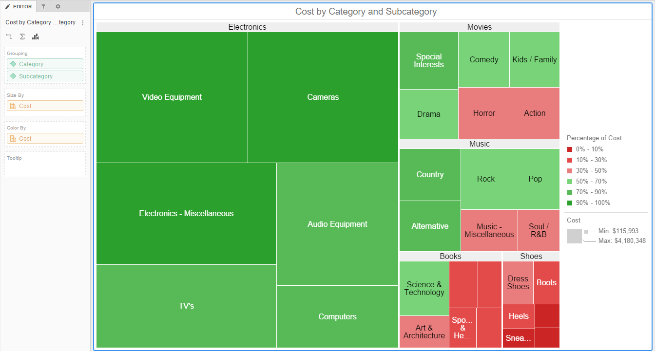
There is nothing about this graphic that I can recommend.

library(dplyr)
#> 
#> Attaching package: 'dplyr'
#> The following objects are masked from 'package:stats':
#> 
#>     filter, lag
#> The following objects are masked from 'package:base':
#> 
#>     intersect, setdiff, setequal, union
library(ggplot2)

e <- data.frame(
  head2 = c(rep("SUB1_A", 7), rep("SUB1_B", 3)),
  head3 = c(rep("SUB2_A", 4), rep("SUB2_B", 3), paste0("TITLE", 1:3)),
  head4 = c(paste0("TITLE", 4:10), rep(NA, 3)),
  value = c(120, 3702, 491, 1738, 1730, 58, 231, 1829, 61, 244)
)

# subtotals
titles <- e |>
  group_by(head2, head3, head4) |>
  summarise(subtotal = sum(value, na.rm = TRUE))
#> `summarise()` has grouped output by 'head2', 'head3'. You can override using
#> the `.groups` argument.
subs <- e |>
  group_by(head2, head3) |>
  summarise(subtotal = sum(value, na.rm = TRUE))
#> `summarise()` has grouped output by 'head2'. You can override using the
#> `.groups` argument.
smalls <- e |>
  group_by(head4) |>
  summarise(subtotal = sum(value, na.rm = TRUE))
smalls <- smalls[complete.cases(smalls), ]
bigs <- e |>
  group_by(head2) |>
  summarise(subtotal = sum(value, na.rm = TRUE))

# sort in numeric order
smalls[8,] <- smalls[1,]
smalls <- smalls[-1,]

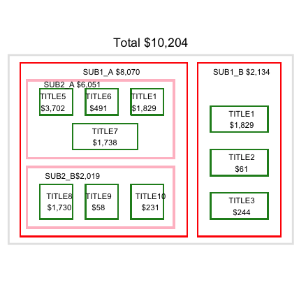
ITEM0 <- paste0("Total $",prettyNum(sum(subs[3]),big.mark = ","))
ITEM1 <- paste0(bigs[1,1]," $",prettyNum(sum(bigs[1,2]),big.mark = ","))
ITEM2 <- paste0(bigs[2,1]," $",prettyNum(sum(bigs[2,2]),big.mark = ","))
ITEM3 <- paste0(subs[1,2]," $",prettyNum(subs[1,3],big.mark = ","))
ITEM4 <- paste0(titles[1,3],"\n$",prettyNum(titles[1,4],big.mark = ","))
ITEM5 <- paste0(titles[2,3],"\n$",prettyNum(titles[2,4],big.mark = ","))
ITEM6 <- paste0(titles[3,3],"\n$",prettyNum(titles[3,4],big.mark = ","))
ITEM7 <- paste0(titles[8,2],"\n$",prettyNum(titles[8,4],big.mark = ","))
ITEM8 <- paste0(titles[4,3],"\n$",prettyNum(titles[4,4],big.mark = ","))
ITEM9 <- paste0(titles[9,2],"\n$",prettyNum(titles[9,4],big.mark = ","))
ITEM10 <- paste0(subs[2,2],"$",prettyNum(subs[2,3],big.mark = ","))
ITEM11 <- paste0(titles[6,3],"\n$",prettyNum(titles[6,4],big.mark = ","))
ITEM12 <- paste0(titles[7,3],"\n$",prettyNum(titles[7,4],big.mark = ","))
ITEM13 <- paste0(titles[5,3],"\n$",prettyNum(titles[5,4],big.mark = ","))
ITEM14 <- paste0(titles[10,2],"\n$",prettyNum(titles[10,4],big.mark = ","))

# cartesian grid to aid locating plot objects
x <- 1:1000
y <- 1:1000
b <- ggplot(,aes(x,y))
b + 
  ggtitle(ITEM0) +
  xlab(NULL) +
  ylab(NULL) +
  geom_rect(xmin = 0, xmax = 640, ymin = 0, ymax = 1000,
            fill = NA, color = "red") +
  geom_rect(xmin = 25, xmax = 590, ymin = 50, ymax = 400,
            fill = NA, color = "pink", size = 1) +
  geom_rect(xmin = 75, xmax = 200, ymin = 100, ymax = 300,
            fill = NA, color = "forestgreen") +
  geom_rect(xmin = 250, xmax = 375, ymin = 100, ymax = 300,
            fill = NA, color = "forestgreen") +
  geom_rect(xmin = 425, xmax = 550, ymin = 100, ymax = 300,
            fill = NA, color = "forestgreen") +
  geom_rect(xmin = 25, xmax = 590, ymin = 450, ymax = 900,
            fill = NA, color = "pink", size = 1) +
  geom_rect(xmin = 200, xmax = 450, ymin = 500, ymax = 650,
            fill = NA, color = "forestgreen") +
  geom_rect(xmin = 75, xmax = 200, ymin = 700, ymax = 850,
            fill = NA, color = "forestgreen") +
  geom_rect(xmin = 250, xmax = 375, ymin = 700, ymax = 850,
            fill = NA, color = "forestgreen") +
  geom_rect(xmin = 425, xmax = 550, ymin = 700, ymax = 850,
            fill = NA, color = "forestgreen") +
  geom_rect(xmin = 680, xmax = 1000, ymin = 0, ymax = 1000,
            fill = NA, color = "red") +
  geom_rect(xmin = 730, xmax = 950, ymin = 100, ymax = 250,
            fill = NA, color = "forestgreen") +
  geom_rect(xmin = 730, xmax = 950, ymin = 350, ymax = 500,
            fill = NA, color = "forestgreen") +
  geom_rect(xmin = 730, xmax = 950, ymin = 600, ymax = 750,
            fill = NA, color = "forestgreen") +
  annotate("text",350,950,label = ITEM1, size = 3) +
  annotate("text",850,950,label = ITEM2, size = 3) +
  annotate("text",200,875,label = ITEM3, size = 3) +
  annotate("text",200,350,label = ITEM10, size = 3) +
  annotate("text",125,775,label = ITEM5, size = 3) +
  annotate("text",300,775,label = ITEM6, size = 3) +
  annotate("text",475,775,label = ITEM7, size = 3) +
  annotate("text",325,575,label = ITEM8, size = 3) +
  annotate("text",150,200,label = ITEM11, size = 3) +
  annotate("text",300,200,label = ITEM12, size = 3) +
  annotate("text",500,200,label = ITEM13, size = 3) +
  annotate("text",850,175,label = ITEM14, size = 3) +
  annotate("text",850,425,label = ITEM9, size = 3) +
  annotate("text",850,675,label = ITEM7, size = 3) +
  theme(plot.title = element_text(hjust = 0.5),
        aspect.ratio = 2/3,
        panel.border = element_rect(color = "gray90",
                                    fill = NA,
                                    size = 2),
        panel.grid = element_line(),
        panel.background = element_blank(),
        axis.title.x=element_blank(),
        axis.text.x=element_blank(),
        axis.title.y=element_blank(),
        axis.text.y=element_blank(),
        axis.title = element_blank(),
        axis.ticks = element_blank()) 
#> Warning: Using `size` aesthetic for lines was deprecated in ggplot2 3.4.0.
#> ℹ Please use `linewidth` instead.
#> This warning is displayed once every 8 hours.
#> Call `lifecycle::last_lifecycle_warnings()` to see where this warning was
#> generated.
#> Warning: The `size` argument of `element_rect()` is deprecated as of ggplot2 3.4.0.
#> ℹ Please use the `linewidth` argument instead.
#> This warning is displayed once every 8 hours.
#> Call `lifecycle::last_lifecycle_warnings()` to see where this warning was
#> generated.

^{Created on 2023-05-15 with reprex v2.0.2}

[RYann]

Thanks man. Guys at SO proposed treemap and it seems to do the trick. That is some great ggplot skills though. Thank you!

[Matthias]

Damn this is what I wanted to suggest right now:

df = tribble(
~"label", ~"value",
"TITLE1",      1829, 
"TITLE2" ,       61, 
"TITLE3",     244, 
"TITLE4",        120,
"TITLE5",       3702,
"TITLE6",        491,
"TITLE7",       1738,
"TITLE8",       1730,
"TITLE9",         58,
"TITLE10",       231) %>% 
  mutate(group = c(rep("SUB1_B", 3),
                   rep("SUB2_A", 4),
                   rep("SUB2_B", 3)),
         size = rep(5, 10))

library(treemap)
# treemap
treemap(df,
        index= c("group", "label"),  # grouping
        type="dens",                 # type = "dens" -> heatmap style
        vSize="size",               # column defining the size of the rectangles 
        vColor = "value",            # column defining the fill colour of rectangles
        fontsize.labels=c(12,8),     # labelsize group, subgroup
        lowerbound.cex.labels = 0,
        palette = "Greens",   
        border.col=c("black","grey"), 
        align.labels=list(
           c("center", "top"), 
           c("left", "center"))
        )