How to use alpha in geom_density, geom_density_ridges, geom_density_ridges_gradient

[Andrzej]

Hi,
I want to make one of the levels of my categorical let's say variable more transparent in order to see distribution underneath.
How do I do it ?
This code is not working properly, how to correct it ?

# Simulate some data
set.seed(123)
n <- 500
datasyn <- data.frame(
  Some_results = rnorm(n),
  Sex = sample(c("female", "male"), size = n, replace = TRUE)
)

# Load ggplot2 library
library(ggplot2)

# Create the plot
ggplot(datasyn, aes(x = Some_results, fill = Sex)) +
  geom_density() +
  scale_fill_manual(values = c("female" = "#FF0000", "male" = "#0000FF")) +
  scale_alpha_manual(values = c("female" = 0.7, "male" = 0.2)) +
  theme(legend.position = "bottom") +
  labs(fill = "Sex")

It gives:

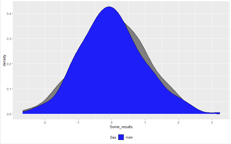
This blue mountain completely obscuring a gray mountain which id situated behind. How to fix it, please ?
Additional thing is that legend is not completed, only male present.

[Matthias]

# Option 1: Include alpha in the aes
ggplot(datasyn, aes(x = Some_results, 
                    fill = Sex, alpha = Sex)) +
  geom_density() +
  scale_fill_manual(values = c("female" = "#FF0000", "male" = "#0000FF")) +
  scale_alpha_manual(values = c("female" = 0.5, "male" = 0.2)) +
  theme(legend.position = "bottom") +
  labs(fill = "Sex")

# Option 2: Define alpha for both
ggplot(datasyn, aes(x = Some_results, 
                    fill = Sex)) +
  geom_density(alpha = 0.25) +
  scale_fill_manual(values = c("female" = "#FF0000", "male" = "#0000FF")) +
  theme(legend.position = "bottom") +
  labs(fill = "Sex")

[Andrzej]

Thank you, this is what I wanted.

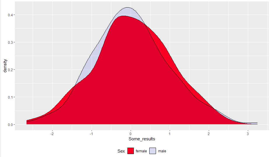
Is it possible to change if possible as well, when density males are in the background and density females are in the foreground to reverse it in the plot and vice-versa ?
How to tweak a bit a legend, I mean how to increase squares and fonts in the legend ?

[Andrzej]

When I use this code:

ggplot(datasyn, aes(x = Some_results,
                    fill = Sex, alpha = Sex)) +
  geom_density() +
  scale_fill_manual(values = c("female" = "#FF0000", "male" = "#0000FF")) +
  scale_alpha_manual(values = c("female" = 0.1, "male" = 1)) +
  theme(legend.position = "bottom") +
  labs(fill = "Sex")

It gives me this:

Male completely covers female.
When I reverse it:

ggplot(datasyn, aes(x = Some_results,
                    fill = Sex, alpha = Sex)) +
  geom_density() +
  scale_fill_manual(values = c("male" = "#0000FF", "female" = "#FF0000")) +
  scale_alpha_manual(values = c("male" = 0.1, "female" = 1)) +
  theme(legend.position = "bottom") +
  labs(fill = "Sex")

It gives me this:

Female not completely covers male. Why is that ?

[Matthias]

This is because changing the order of the colours just doesn't change the stacking order, female is still at the bottom, male on top. (Because they are drawn in alphabetic order female, then male)
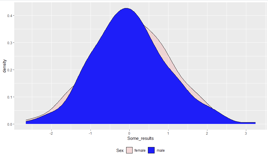
With a high enough transparency (alpha <= 0.5) the effect shouldn't be so visible (okay the mixing is still a bit different).
What you can do is to reverse the stacking order using fct_rev() from the forcats package.

ggplot(datasyn, aes(x = Some_results, 
                    fill = forcats::fct_rev(Sex) )) +
  geom_density(alpha = 0.7) +
  scale_fill_manual("Sex",
                    values = c("female" = "#FF0000", "male" = "#0000FF")) +
  theme(legend.position = "bottom") +
  labs(fill = "Sex") +
  theme(legend.key.size = unit(2,"line"),       # size of legend items
        legend.text = element_text(size = 14),  # size of legend labels
        legend.title = element_text(size = 16,
                                    face = "bold")) # size of legend header

When you wnat to keep the alpha differentially you need to add the same for the alpha.
See also the settings for bigger legend.
For more control check this: Legend guide — guide_legend • ggplot2