I have questionnaire data of the kind "check all options that apply", and I wonder how to analyze it properly such that:
- I account for by-subject nature of the data
- I'll be able to compare different options against each other
- I get estimates
- I get confidence intervals
I've found that Cochran's Q & McNemar Chi-squared tests might be good options. However, I'm not sure what would be a proper analysis that achieves all the requirements I listed above.
To anchor my question with data, please consider the following reproducible example.
I have distributed a questionnaire in which I asked people a single question:
here are some common types of food, please mark all the types you like (all that apply):
☐ broccoli
☐ pizza
☐ pie
☐ spinach
☐ sausage
☐ orange
☐ blueberries muffin
☐ chocolate cake
☐ pasta
☐ fried potatoes
☐ burrito
☐ mac and cheese
The data looks like that:
# just run the following to simulate the data
library(tidyverse)
library(ids)

food_table <-
  tibble::tribble(
                ~food, ~prop,
           "broccoli", 0.482,
              "pizza",  0.82,
                "pie", 0.299,
            "spinach", 0.234,
            "sausage",   0.4,
             "orange",  0.05,
 "blueberries_muffin", 0.269,
     "chocolate_cake", 0.063,
              "pasta", 0.025,
     "fried_potatoes", 0.122,
            "burrito", 0.117,
     "mac_and_cheese", 0.032
 )

rowwise_data <-
  food_table %>%
  mutate(binomial_data = map(.x = prop, .f = ~rbinom(n = 3000, size = 1, prob = .x))) %>%
  select(-prop) %>%
  pivot_wider(names_from = food, values_from = binomial_data) %>%
  unnest(cols = everything()) %>%
  mutate(ids = uuid(n = nrow(.)), .before = everything())

rowwise_data
#> # A tibble: 3,000 x 13
#>    ids              broccoli pizza   pie spinach sausage orange blueberries_muf~
#>    <chr>               <int> <int> <int>   <int>   <int>  <int>            <int>
#>  1 02d95100-719e-4~        0     1     0       0       1      0                0
#>  2 fd1f1759-721d-4~        0     0     0       1       1      0                0
#>  3 fa33ea76-6149-4~        0     1     1       0       0      0                0
#>  4 6664d209-766e-4~        0     1     0       0       0      0                0
#>  5 db9b3466-d932-4~        1     1     1       1       1      0                0
#>  6 22edb5dc-4519-4~        1     1     0       0       1      0                0
#>  7 3f05a385-0dcc-4~        0     1     0       1       1      0                0
#>  8 909f2f1d-c37b-4~        0     1     0       0       0      0                0
#>  9 3160fbcf-b8d0-4~        0     1     1       0       1      0                1
#> 10 ce204abf-3960-4~        1     1     0       0       0      0                0
#> # ... with 2,990 more rows, and 5 more variables: chocolate_cake <int>,
#> #   pasta <int>, fried_potatoes <int>, burrito <int>, mac_and_cheese <int>
Created on 2022-01-27 by the reprex package (v2.0.1.9000)
We can see that each row pertains to one individual who answered the questionnaire. We also have one column per each option, and values 0 or 1 denoting whether the person checked that option or not.
How to statistically model this data?
option A -- using `binom.test()`
One option would be to run `stats::binom.test()` on each column. Doing so we will get estimates and confidence intervals for each *option* separately, and regardless of survey respondents (i.e., per option across all respondents). Here's an example of such analysis:separate_binom_test <-
rowwise_data %>%
pivot_longer(-ids) %>%
group_by(name) %>%
nest() %>%
mutate(n_of_success = map_int(.x = data, .f = ~ sum(.x$value)),
n_of_trials = map_int(.x = data, .f = ~ length(.x$value)),
test_result = map2(.x = n_of_success, .y = n_of_trials, .f = ~binom.test(.x, .y) %>% broom::tidy())) %>%
select(name, test_result) %>%
unnest_wider(test_result)
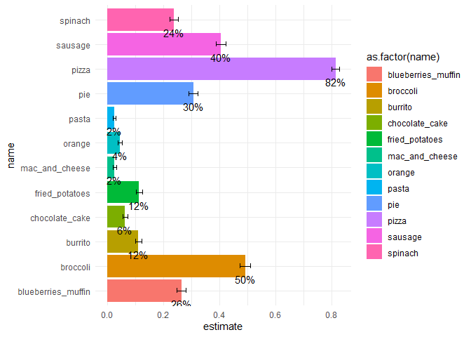
We can visualize this analysis:
separate_binom_test %>%
  ggplot(aes(x = name, y = estimate, fill = as.factor(name))) +
  geom_bar(stat = "identity") +
  geom_errorbar(aes(ymin = conf.low, ymax = conf.high), width = 0.2) +
  geom_text(aes(label = scales::percent(estimate, 2)), vjust = 2) +
  coord_flip() +
  theme_minimal()

Created on 2022-01-27 by the reprex package (v2.0.1.9000)
We got:
✓ estimates
✓ confidence intervals
We didn't get:
✗ accounting for by-subject nature of the data
✗ being able to compare different options against each other (well kind of yes, we can compare CIs, but not real contrasts...)
option B -- using Cochran's Q / McNemar Chi-squared tests
library(rstatix)

rowwise_data %>%
  pivot_longer(-ids) %>%
  mutate(across(value, as.factor)) %>%
  group_by(ids) %>%
  ungroup() %>%
  pairwise_mcnemar_test(., value ~ name|ids)
#> # A tibble: 66 x 6
#>    group1             group2                 p     p.adj p.adj.signif method
#>  * <chr>              <chr>              <dbl>     <dbl> <chr>        <chr>
#>  1 blueberries_muffin broccoli       6.98e- 73 4.61e- 71 ****         McNemar t~
#>  2 blueberries_muffin burrito        7.76e- 44 5.12e- 42 ****         McNemar t~
#>  3 blueberries_muffin chocolate_cake 7.55e- 99 4.98e- 97 ****         McNemar t~
#>  4 blueberries_muffin fried_potatoes 5.43e- 41 3.58e- 39 ****         McNemar t~
#>  5 blueberries_muffin mac_and_cheese 3.8 e-132 2.51e-130 ****         McNemar t~
#>  6 blueberries_muffin orange         1.08e- 96 7.13e- 95 ****         McNemar t~
#>  7 blueberries_muffin pasta          7.79e-132 5.14e-130 ****         McNemar t~
#>  8 blueberries_muffin pie            1.37e-  3 9.04e-  2 ns           McNemar t~
#>  9 blueberries_muffin pizza          2.43e-316 1.60e-314 ****         McNemar t~
#> 10 blueberries_muffin sausage        1.23e- 28 8.12e- 27 ****         McNemar t~
#> # ... with 56 more rows
Created on 2022-01-27 by the reprex package (v2.0.1.9000)
In contrast to option A, here we got:
✓ accounting for by-subject nature of the data
✓ being able to compare different options against each other
but not
✗ estimates
✗ confidence intervals
In addition, with this option B, I'm not sure how to visualize the data.
Bottom line
Options A vs. B offer different (competing?) ways to model the data. I do not know how to combine the two or if it's statistically okay to do. I feel more comfortable with option B, but then again: I don't have estimates and CIs and thus am limited with visualizing ![]()
Any idea how to reconcile a unified analysis?
Thanks!
