How to specify the area of a grid cell drawn by geom_sf()?

Wyno0 · May 24, 2024, 4:00pm

Hello,
I'm trying to plot my results for the tree crowns I detected in a part of the Canadian boreal forest. And I would like to know how to know how much represents a cell of the grid that we see appearing in font of my plot. Can I change the value of the cells so that they represent 1ha, 1/2ha, 1/10ha, etc?

ggplot() +
  geom_sf(data = crowns4_crop, aes(fill = convhull_area)) +
  scale_fill_viridis_c(name = "Crown area (m²)") + 
  geom_sf(data = ttops4_crop, color = "red", pch = 3, size = 2, show.legend = FALSE)  + 
  theme(axis.text = element_blank(),
        axis.title = element_blank(),
        axis.ticks = element_blank(),
        plot.title = element_text(hjust = 0.5)) + 
  labs(title = "Crown & Tree")

Thanks!
Lea

dromano · May 24, 2024, 9:35pm

Do you mean a rectangle formed by the white horizontal and vertical lines?

What are the units you use in the crowns4_crop table for the coordinates of the points? Are they latitude and longitude?

Wyno0 · May 27, 2024, 3:03pm

Exactly I meant that, and yes my coordinates for "crowns4_crop" are in latitude and longitude

dromano · May 27, 2024, 3:55pm

To be precise, it would be best to share the data, but it might be enough to just run the same code but remove the line

and share the resulting image so that the range of latitude and longitude is clear — is that something you can do?

jrkrideau · May 27, 2024, 4:18pm

A handy way to supply some sample data is the dput() function. In the case of a large dataset something like dput(head(mydata, 100)) should supply the data we need. Just do dput(mydata) where mydata is your data. Copy the output and paste it here between
```

```

Wyno0 · May 27, 2024, 4:30pm

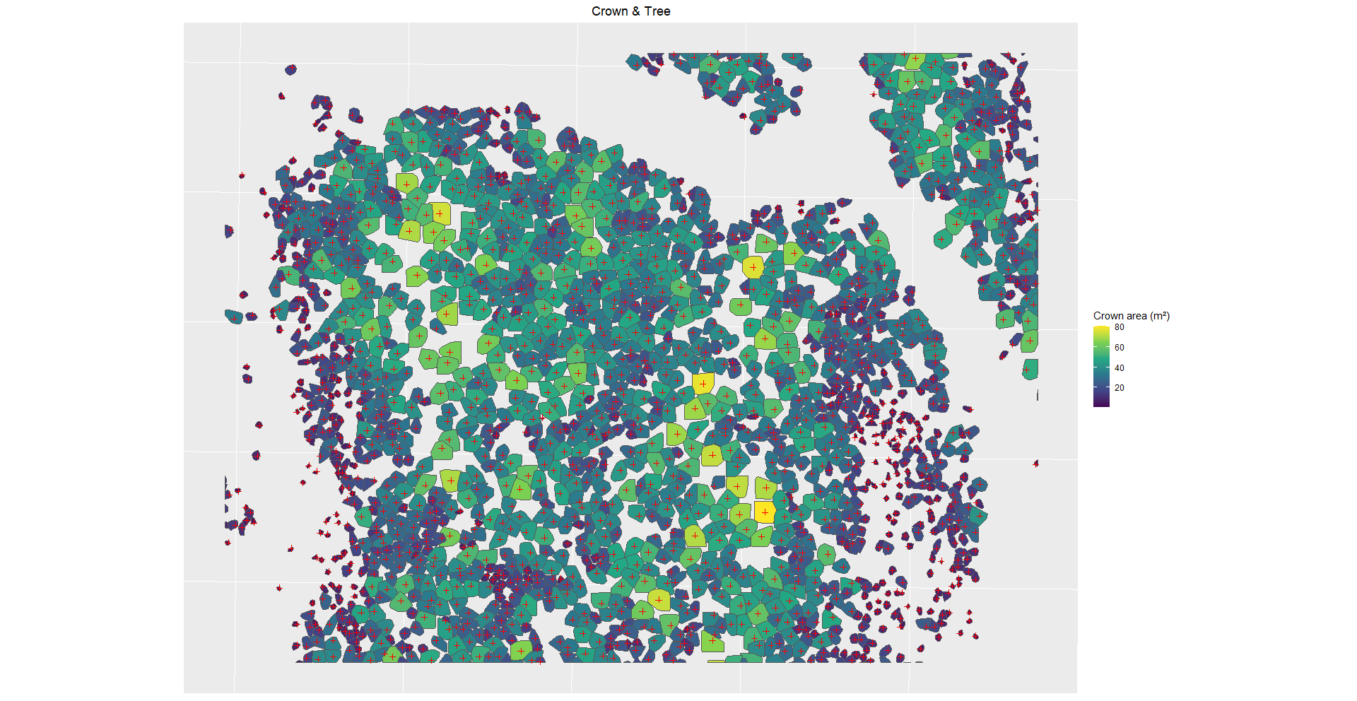
Hi, here is the result, I only did for 10 because it's a lot of information already. Let me know if you need more.

dput(head(crowns4_crop, 5))
structure(list(treeID = c(7154, 7174, 7175, 7199, 7200), Z = c(19.74775, 
20.08075, 17.71525, 15.27575, 13.89975), npoints = c(473L, 394L, 
311L, 432L, 323L), convhull_area = c(43.898, 33.437, 19.422, 
36.496, 28.327), geometry = structure(list(structure(list(structure(c(255833.4125, 
255833.23675, 255831.993001074, 255834.594286062, 255833.4125, 
5501574.16775, 5501574.298, 5501575.25083612, 5501575.25083612, 
5501574.16775), dim = c(5L, 2L))), class = c("XY", "POLYGON", 
"sfg")), structure(list(structure(c(255856.27475, 255855.8075, 
255854.6055, 255853.493676096, 255858.401473068, 255856.27475, 
5501573.72825, 5501573.68075, 5501574.07975, 5501575.25083612, 
5501575.25083612, 5501573.72825), dim = c(6L, 2L))), class = c("XY", 
"POLYGON", "sfg")), structure(list(structure(c(255866.404, 255865.93525, 
255865.393, 255863.785, 255863.205, 255863.033976154, 255866.481341375, 
255866.404, 5501575.19, 5501574.92275, 5501574.61925, 5501574.72925, 
5501575.09725, 5501575.25083612, 5501575.25083612, 5501575.19
), dim = c(8L, 2L))), class = c("XY", "POLYGON", "sfg")), structure(list(
    structure(c(255907.4005, 255906.61925, 255906.17825, 255904.27425, 
    255901.62325, 255901.142, 255900.59225, 255900.586204727, 
    255908.506793168, 255907.4005, 5501574.0445, 5501573.728, 
    5501573.68025, 5501573.523, 5501574.30775, 5501574.68175, 
    5501575.198, 5501575.25083612, 5501575.25083612, 5501574.0445
    ), dim = c(10L, 2L))), class = c("XY", "POLYGON", "sfg")), 
    structure(list(structure(c(255935.07475, 255934.33925, 255934.28225, 
    255933.333063605, 255935.154217763, 255935.154217763, 255935.07475, 
    5501574.15, 5501574.27075, 5501574.311, 5501575.25083612, 
    5501575.25083612, 5501574.14661042, 5501574.15), dim = c(7L, 
    2L))), class = c("XY", "POLYGON", "sfg"))), class = c("sfc_POLYGON", 
"sfc"), precision = 0, bbox = structure(c(xmin = 255831.993001074, 
ymin = 5501573.523, xmax = 255935.154217763, ymax = 5501575.25083612
), class = "bbox"), crs = structure(list(input = "EPSG:2949", 
    wkt = "PROJCRS[\"NAD83(CSRS) / MTM zone 7\",\n    BASEGEOGCRS[\"NAD83(CSRS)\",\n        DATUM[\"NAD83 Canadian Spatial Reference System\",\n            ELLIPSOID[\"GRS 1980\",6378137,298.257222101,\n                LENGTHUNIT[\"metre\",1]]],\n        PRIMEM[\"Greenwich\",0,\n            ANGLEUNIT[\"degree\",0.0174532925199433]],\n        ID[\"EPSG\",4617]],\n    CONVERSION[\"MTM zone 7\",\n        METHOD[\"Transverse Mercator\",\n            ID[\"EPSG\",9807]],\n        PARAMETER[\"Latitude of natural origin\",0,\n            ANGLEUNIT[\"degree\",0.0174532925199433],\n            ID[\"EPSG\",8801]],\n        PARAMETER[\"Longitude of natural origin\",-70.5,\n            ANGLEUNIT[\"degree\",0.0174532925199433],\n            ID[\"EPSG\",8802]],\n        PARAMETER[\"Scale factor at natural origin\",0.9999,\n            SCALEUNIT[\"unity\",1],\n            ID[\"EPSG\",8805]],\n        PARAMETER[\"False easting\",304800,\n            LENGTHUNIT[\"metre\",1],\n            ID[\"EPSG\",8806]],\n        PARAMETER[\"False northing\",0,\n            LENGTHUNIT[\"metre\",1],\n            ID[\"EPSG\",8807]]],\n    CS[Cartesian,2],\n        AXIS[\"easting (E(X))\",east,\n            ORDER[1],\n            LENGTHUNIT[\"metre\",1]],\n        AXIS[\"northing (N(Y))\",north,\n            ORDER[2],\n            LENGTHUNIT[\"metre\",1]],\n    USAGE[\n        SCOPE[\"Engineering survey, topographic mapping.\"],\n        AREA[\"Canada - Quebec - between 72°W and 69°W.\"],\n        BBOX[45.01,-72,61.8,-69]],\n    ID[\"EPSG\",2949]]"), class = "crs"), n_empty = 0L)), sf_column = "geometry", agr = structure(c(treeID = NA_integer_, 
Z = NA_integer_, npoints = NA_integer_, convhull_area = NA_integer_
), levels = c("constant", "aggregate", "identity"), class = "factor"), row.names = c(5886L, 
5900L, 5901L, 5918L, 5919L), class = c("sf", "data.table", "data.frame"
))

Wyno0 · May 27, 2024, 4:32pm

Hello, here is the result :

Wyno0 · May 27, 2024, 4:34pm

Hi, here is the result (I only did for 5 because it's a lot of information already) :

dput(head(crowns4_crop, 5))
structure(list(treeID = c(7154, 7174, 7175, 7199, 7200), Z = c(19.74775, 
20.08075, 17.71525, 15.27575, 13.89975), npoints = c(473L, 394L, 
311L, 432L, 323L), convhull_area = c(43.898, 33.437, 19.422, 
36.496, 28.327), geometry = structure(list(structure(list(structure(c(255833.4125, 
255833.23675, 255831.993001074, 255834.594286062, 255833.4125, 
5501574.16775, 5501574.298, 5501575.25083612, 5501575.25083612, 
5501574.16775), dim = c(5L, 2L))), class = c("XY", "POLYGON", 
"sfg")), structure(list(structure(c(255856.27475, 255855.8075, 
255854.6055, 255853.493676096, 255858.401473068, 255856.27475, 
5501573.72825, 5501573.68075, 5501574.07975, 5501575.25083612, 
5501575.25083612, 5501573.72825), dim = c(6L, 2L))), class = c("XY", 
"POLYGON", "sfg")), structure(list(structure(c(255866.404, 255865.93525, 
255865.393, 255863.785, 255863.205, 255863.033976154, 255866.481341375, 
255866.404, 5501575.19, 5501574.92275, 5501574.61925, 5501574.72925, 
5501575.09725, 5501575.25083612, 5501575.25083612, 5501575.19
), dim = c(8L, 2L))), class = c("XY", "POLYGON", "sfg")), structure(list(
    structure(c(255907.4005, 255906.61925, 255906.17825, 255904.27425, 
    255901.62325, 255901.142, 255900.59225, 255900.586204727, 
    255908.506793168, 255907.4005, 5501574.0445, 5501573.728, 
    5501573.68025, 5501573.523, 5501574.30775, 5501574.68175, 
    5501575.198, 5501575.25083612, 5501575.25083612, 5501574.0445
    ), dim = c(10L, 2L))), class = c("XY", "POLYGON", "sfg")), 
    structure(list(structure(c(255935.07475, 255934.33925, 255934.28225, 
    255933.333063605, 255935.154217763, 255935.154217763, 255935.07475, 
    5501574.15, 5501574.27075, 5501574.311, 5501575.25083612, 
    5501575.25083612, 5501574.14661042, 5501574.15), dim = c(7L, 
    2L))), class = c("XY", "POLYGON", "sfg"))), class = c("sfc_POLYGON", 
"sfc"), precision = 0, bbox = structure(c(xmin = 255831.993001074, 
ymin = 5501573.523, xmax = 255935.154217763, ymax = 5501575.25083612
), class = "bbox"), crs = structure(list(input = "EPSG:2949", 
    wkt = "PROJCRS[\"NAD83(CSRS) / MTM zone 7\",\n    BASEGEOGCRS[\"NAD83(CSRS)\",\n        DATUM[\"NAD83 Canadian Spatial Reference System\",\n            ELLIPSOID[\"GRS 1980\",6378137,298.257222101,\n                LENGTHUNIT[\"metre\",1]]],\n        PRIMEM[\"Greenwich\",0,\n            ANGLEUNIT[\"degree\",0.0174532925199433]],\n        ID[\"EPSG\",4617]],\n    CONVERSION[\"MTM zone 7\",\n        METHOD[\"Transverse Mercator\",\n            ID[\"EPSG\",9807]],\n        PARAMETER[\"Latitude of natural origin\",0,\n            ANGLEUNIT[\"degree\",0.0174532925199433],\n            ID[\"EPSG\",8801]],\n        PARAMETER[\"Longitude of natural origin\",-70.5,\n            ANGLEUNIT[\"degree\",0.0174532925199433],\n            ID[\"EPSG\",8802]],\n        PARAMETER[\"Scale factor at natural origin\",0.9999,\n            SCALEUNIT[\"unity\",1],\n            ID[\"EPSG\",8805]],\n        PARAMETER[\"False easting\",304800,\n            LENGTHUNIT[\"metre\",1],\n            ID[\"EPSG\",8806]],\n        PARAMETER[\"False northing\",0,\n            LENGTHUNIT[\"metre\",1],\n            ID[\"EPSG\",8807]]],\n    CS[Cartesian,2],\n        AXIS[\"easting (E(X))\",east,\n            ORDER[1],\n            LENGTHUNIT[\"metre\",1]],\n        AXIS[\"northing (N(Y))\",north,\n            ORDER[2],\n            LENGTHUNIT[\"metre\",1]],\n    USAGE[\n        SCOPE[\"Engineering survey, topographic mapping.\"],\n        AREA[\"Canada - Quebec - between 72°W and 69°W.\"],\n        BBOX[45.01,-72,61.8,-69]],\n    ID[\"EPSG\",2949]]"), class = "crs"), n_empty = 0L)), sf_column = "geometry", agr = structure(c(treeID = NA_integer_, 
Z = NA_integer_, npoints = NA_integer_, convhull_area = NA_integer_
), levels = c("constant", "aggregate", "identity"), class = "factor"), row.names = c(5886L, 
5900L, 5901L, 5918L, 5919L), class = c("sf", "data.table", "data.frame"
))

dromano · May 27, 2024, 5:52pm

Thanks, Léa: This looks like a different image and the data you shared was in meters rather than latitude and longitude — did you use slightly different code (aside from my suggestion) to produce this image?

Wyno0 · May 27, 2024, 6:00pm

It's the same data and same code, just a different window because I draw it myself every time and doesn't save it (because it doesn't matter if it's the same window or not)

dromano · May 27, 2024, 6:01pm

Could you say more? I'm not sure what you mean by "window".

jrkrideau · May 27, 2024, 6:02pm

Thanks for the data but am I misreading your code?

It looks like you are calling 2 datasets

crowns4_crop
ttops4_crop

but unless I am completely missing something I am only seeing one in your post.

Wyno0 · May 27, 2024, 6:05pm

Sure, the raw data are LiDAR tiles of 1km² so every result that I get (crowns and ttops) are also a tile of 1km². But to make it more visible I crop the results using the function drawExtent(). What I call the window is the crop version of the tile

dromano · May 27, 2024, 6:28pm

Thanks, that's helpful to know.

Could you post the output from running just this?

crowns4_crop

Wyno0 · May 27, 2024, 6:35pm

Of course, here you go :

crowns4_crop
Simple feature collection with 1686 features and 4 fields
Geometry type: POLYGON
Dimension:     XY
Bounding box:  xmin: 255639.7 ymin: 5501330 xmax: 255948.2 ymax: 5501573
Projected CRS: NAD83(CSRS) / MTM zone 7
First 10 features:
     treeID        Z npoints convhull_area                       geometry
5912   7192 14.56825     404        33.226 POLYGON ((255940.7 5501573,...
5924   7209 21.03800     476        37.700 POLYGON ((255918.7 5501573,...
5935   7226 19.02475     334        22.805 POLYGON ((255840.8 5501573,...
5936   7227 19.37825     571        44.054 POLYGON ((255924.7 5501572,...
5937   7228 17.10525     373        31.217 POLYGON ((255933 5501571, 2...
5938   7229 14.32125     355        29.815 POLYGON ((255947.9 5501573,...
5948   7245 19.88075     402        32.013 POLYGON ((255854.5 5501572,...
5954   7254 15.49200     176        15.205 POLYGON ((255664.8 5501573,...
5960   7264 18.83150     261        18.040 POLYGON ((255839.9 5501572,...
5964   7274 13.00500     237        16.096 POLYGON ((255660.5 5501570,...

dromano · May 27, 2024, 7:01pm

Does this work for you? I used the value of the bounding box from the output from crowns4_crop that you shared, and I used the EPSG number that corresponds to MTM zone 7 (2949):

# function that calculates width of square whose area is 1/d ha
ha_fraction_width <- 
  function(d){
    100 / sqrt(d)
  } 

# example: width of square of area 1/4 ha
ha_width <- ha_fraction_width(4)

ggplot() +
  geom_sf(data = crowns4_crop, aes(fill = convhull_area)) +
  scale_fill_viridis_c(name = "Crown area (m²)") + 
  geom_sf(data = ttops4_crop, color = "red", pch = 3, size = 2, show.legend = FALSE)  +
  coord_sf(datum = st_crs(2949)) +
  scale_x_continuous(breaks = seq(255639.7, 255948.2, by = ha_width)) +
  scale_y_continuous(breaks = seq(5501330, 5501573, by = ha_width)) +
  theme(axis.text = element_blank(),
        axis.title = element_blank(),
        axis.ticks = element_blank(),
        plot.title = element_text(hjust = 0.5)) + 
  labs(title = "Crown & Tree")

Wyno0 · May 27, 2024, 7:40pm

It works, and if I understand correctly, this code means that each cell of the grid is 1/4 ha?

dromano · May 27, 2024, 7:56pm

Yes, for d = 4, and you can change d to whatever value you prefer.

dromano · May 28, 2024, 1:28pm

Léa: Would you mind if I changed the title of your original post to reflect it contents more closely?

Wyno0 · May 29, 2024, 1:54pm

I don't mind at all, do as your please