I have 32 months of data, and I'm trying out different models for testing the forecasting of unit transitions to dead state "X" for months 13-32, by training from transitions data for months 1-12. I then compare the forecasts with the actual data for months 13-32. The data represents the unit migration of a beginning population into the dead state over 32 months. Not all beginning units die off, only a portion. I understand that 12 months of data for model training isn't much and that forecasting for 20 months from those 12 months should result in a wide distribution of outcomes, those are the real-world limitations I usually grapple with.
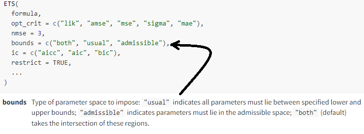
I am using the fable package ETS model and would like to know how, or if it's possible, to set bounds for outputs when running simulations based on ETS. When I go to https://fable.tidyverts.org/reference/ETS.html to research setting bounds, the bounds argument as duplicated in the image below (perhaps I misunderstand what is meant by "bounds"), but those instructions don't say how to actually specify the lower and upper bounds:
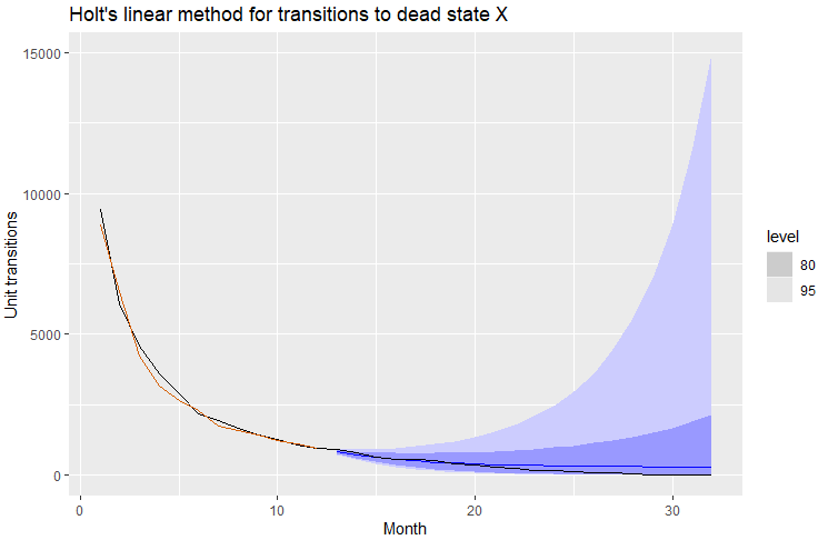
When I run ETS on my data and plot out the forecast I get the following, where the forecast mean (in blue) at least visually reasonably hews to the actual data for those same months 13-32 (in black)(I have run other tests of residuals and autocorrelations, as well as run the benchmark methods recommended in the book, and this Holt's linaer method looks fine based on those tests):
However, when I run simulations using that ETS model (simulation code posted at bottom), I often get a maximum of transitions into dead state X for the forecast horizon (aggregate forecasted transitions during months 13-32) in excess of the beginning number of elements, which totals 60,000. In other words, there is no real-world scenario where transitions to dead state can exceed the beginning population! Is there a way to set an upper bound on the forecast distribution and the simulations so the total forecast doesn't exceed the cap of 60,000 possible transitions?
I use a log-transformation of the data to prevent the forecast from falling negative. Negative value transitions aren't a real-world possibility for this data.
Below is the code for generating the above, including the dataset:
library(dplyr)
library(fabletools)
library(fable)
library(feasts)
library(ggplot2)
library(tidyr)
library(tsibble)

# my data
data <- data.frame(
  Month =c(1:32),
  StateX=c(
    9416,6086,4559,3586,2887,2175,1945,1675,1418,1259,1079,940,923,776,638,545,547,510,379,
    341,262,241,168,155,133,76,69,45,17,9,5,0
  )
) %>%
  as_tsibble(index = Month)

# fit the model to my data, generate forecast for months 13-32, and plot
fit <- data[1:12,] |> model(ETS(log(StateX) ~ error("A") + trend("A") + season("N")))
fc <- fit |> forecast(h = 20)
fc |>
  autoplot(data) +
  geom_line(aes(y = .fitted), col="#D55E00",
            data = augment(fit)) +
  labs(y="Unit transitions", title="Holt's linear method for transitions to dead state X") +
  guides(colour = "none")

# run simulations and show aggregate nbr of transitions for months 13-32
sim <- fit %>% generate(h = 20, times = 5000, bootstrap = TRUE)
agg_sim <- sim %>% group_by(.rep) %>% summarise(sum_FC = sum(.sim),.groups = 'drop')
max(agg_sim[,"sum_FC"])
Referred here by Forecasting: Principles and Practice, by Rob J Hyndman and George Athanasopoulos

