Hi @mtoufiq,
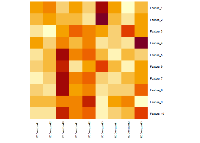
Here is some code to read your data matrix and reshape it into a new data.frame. I wasn't able to produce your desired output since its not clear to me how you want the data "summarized" or subsetted.
Adding annotation text to the left-hand side of heatmap() output is not easy - other forum members may have some ideas.
suppressPackageStartupMessages(library(tidyverse))

input.df <- structure(
  list(
    'E0 Compound 1' = c(
      0.028643405,
      -0.170597892,
      -0.133431392,
      0.362602406,
      0.65949239,
      0.129862499,
      0.308021483,
      0.191411185,
      -0.408706956,
      0.148431726
    ),
    'E0 Compound 2' = c(
      0.312575401,
      0.08023047,
      -0.952555759,
      -0.087364689,
      2.492343411,
      0.594530215,
      1.257403638,
      -0.005561728,
      -0.372470805,
      0.019060103
    ),
    'E0 Compound 3' = c(
      -1.088143295,
      -0.282639558,
      1.283875318,
      0.436371912,
      7.875801388,
      3.888644506,
      4.851154755,
      2.112242014,
      0.35468163,
      2.231527721
    ),
    'P0 Compound 1' = c(
      0.0487268,
      -0.00328775,
      2.07844595,
      -0.014618298,
      4.735091392,
      -0.220327528,
      2.872283004,
      0.77093127,
      0.168573042,
      1.237777012
    ),
    'P0 Compound 2' = c(
      -1.125845192,
      -0.801624332,
      1.669743718,
      0.415204306,
      4.986942824,
      1.496006014,
      3.336380665,
      1.162817817,
      1.491530314,
      1.484104864
    ),
    'P0 Compound 3' = c(
      2.082646448,
      2.708726878,
      1.256777456,
      -0.491426149,
      2.459378121,
      2.981105751,
      0.974149318,
      -0.222540059,
      -1.407150779,
      -0.147072039
    ),
    'R0 Compound 1' = c(
      -0.326900367,
      -0.362728527,
      0.509587017,
      -0.165210608,
      -0.283082038,
      0.753676032,
      0.360670113,
      0.037390082,
      0.103973162,
      0.311012902
    ),
    'R0 Compound 2' = c(
      -2.793220245,
      -0.826729075,
      2.509040525,
      -0.344938067,
      2.868355513,
      -1.025542457,
      1.875640888,
      0.096367013,
      0.233463623,
      0.646241163
    ),
    'R0 Compound 3' = c(
      -0.415009733,
      0.089591797,
      1.245990797,
      1.529969694,
      1.696672088,
      1.578365108,
      2.218401723,
      1.391261115,
      -1.716869822,
      1.869097396
    )
  ),
  class = "data.frame",
  row.names = c(
    "Feature_1",
    "Feature_2",
    "Feature_3",
    "Feature_4",
    "Feature_5",
    "Feature_6",
    "Feature_7",
    "Feature_8",
    "Feature_9",
    "Feature_10"))

input.df
#>            E0 Compound 1 E0 Compound 2 E0 Compound 3 P0 Compound 1
#> Feature_1     0.02864341   0.312575401    -1.0881433    0.04872680
#> Feature_2    -0.17059789   0.080230470    -0.2826396   -0.00328775
#> Feature_3    -0.13343139  -0.952555759     1.2838753    2.07844595
#> Feature_4     0.36260241  -0.087364689     0.4363719   -0.01461830
#> Feature_5     0.65949239   2.492343411     7.8758014    4.73509139
#> Feature_6     0.12986250   0.594530215     3.8886445   -0.22032753
#> Feature_7     0.30802148   1.257403638     4.8511548    2.87228300
#> Feature_8     0.19141119  -0.005561728     2.1122420    0.77093127
#> Feature_9    -0.40870696  -0.372470805     0.3546816    0.16857304
#> Feature_10    0.14843173   0.019060103     2.2315277    1.23777701
#>            P0 Compound 2 P0 Compound 3 R0 Compound 1 R0 Compound 2
#> Feature_1     -1.1258452     2.0826464   -0.32690037   -2.79322025
#> Feature_2     -0.8016243     2.7087269   -0.36272853   -0.82672908
#> Feature_3      1.6697437     1.2567775    0.50958702    2.50904053
#> Feature_4      0.4152043    -0.4914261   -0.16521061   -0.34493807
#> Feature_5      4.9869428     2.4593781   -0.28308204    2.86835551
#> Feature_6      1.4960060     2.9811058    0.75367603   -1.02554246
#> Feature_7      3.3363807     0.9741493    0.36067011    1.87564089
#> Feature_8      1.1628178    -0.2225401    0.03739008    0.09636701
#> Feature_9      1.4915303    -1.4071508    0.10397316    0.23346362
#> Feature_10     1.4841049    -0.1470720    0.31101290    0.64624116
#>            R0 Compound 3
#> Feature_1     -0.4150097
#> Feature_2      0.0895918
#> Feature_3      1.2459908
#> Feature_4      1.5299697
#> Feature_5      1.6966721
#> Feature_6      1.5783651
#> Feature_7      2.2184017
#> Feature_8      1.3912611
#> Feature_9     -1.7168698
#> Feature_10     1.8690974

# To get close to image posted
heatmap(as.matrix(input.df), Rowv=NA, Colv=NA, revC=TRUE, cexRow=0.7, cexCol=0.6)
input.df %>%
  rownames_to_column("Feature") %>%
  pivot_longer(cols=contains("Compound")) %>%
  mutate(Feature = as.factor(Feature),
         Subject = as.factor(str_sub(name, start=1, end=2)),
         Compound = as.factor(str_sub(name, start=4, end=13)),
         Compound = as.factor(str_replace(Compound, " ", "_"))) %>%
  select(-name) -> new.df

new.df
#> # A tibble: 90 × 4
#>    Feature     value Subject Compound
#>    <fct>       <dbl> <fct>   <fct>
#>  1 Feature_1  0.0286 E0      Compound_1
#>  2 Feature_1  0.313  E0      Compound_2
#>  3 Feature_1 -1.09   E0      Compound_3
#>  4 Feature_1  0.0487 P0      Compound_1
#>  5 Feature_1 -1.13   P0      Compound_2
#>  6 Feature_1  2.08   P0      Compound_3
#>  7 Feature_1 -0.327  R0      Compound_1
#>  8 Feature_1 -2.79   R0      Compound_2
#>  9 Feature_1 -0.415  R0      Compound_3
#> 10 Feature_2 -0.171  E0      Compound_1
#> # … with 80 more rows
str(new.df)
#> tibble [90 × 4] (S3: tbl_df/tbl/data.frame)
#>  $ Feature : Factor w/ 10 levels "Feature_1","Feature_10",..: 1 1 1 1 1 1 1 1 1 3 ...
#>  $ value   : num [1:90] 0.0286 0.3126 -1.0881 0.0487 -1.1258 ...
#>  $ Subject : Factor w/ 3 levels "E0","P0","R0": 1 1 1 2 2 2 3 3 3 1 ...
#>  $ Compound: Factor w/ 3 levels "Compound_1","Compound_2",..: 1 2 3 1 2 3 1 2 3 1 ...
Created on 2022-06-04 by the reprex package (v2.0.1)
Hope this helps.