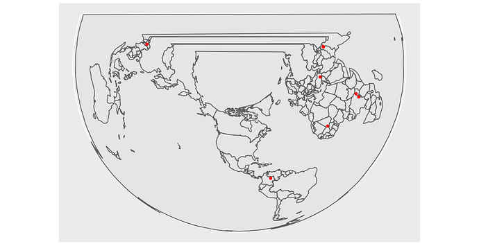
How to project CRS correctly

Hi everyone,

I am working on a project where I map conflict data (csv format, geometry type = points) on polygons (kml files). Both layers are data.frames and share the same CRS (+proj=longlat +datum=WGS84 +no_defs).

The mapping seems to work (see code) however, I receive the following warning message:
"although coordinates are longitude/latitude, st_intersects assumes that they are planar"

I assume this warning appears because the CRS of the two layers is unprojected. Could that be the case and if yes, how can I project it?

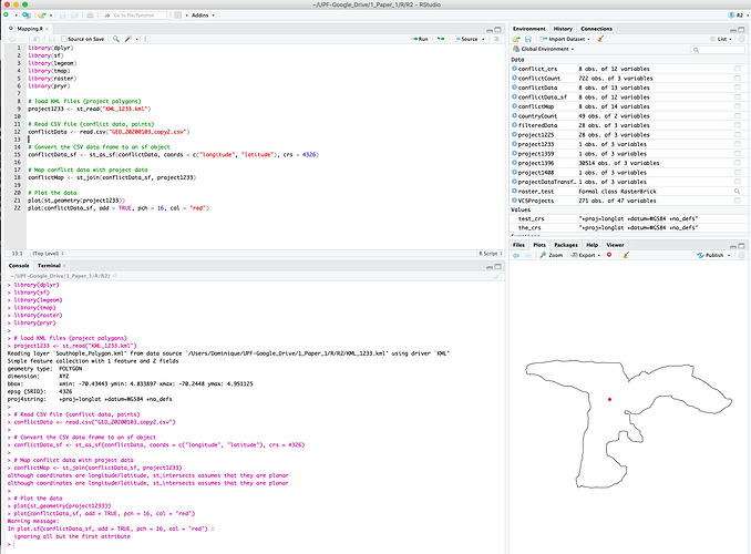
Please find attached a screenshot of my workspace and I am sharing the three files (csv, kml and script) here: https://www.dropbox.com/sh/eisoxjbyojevlzs/AABW6A0GjELt1pOJXb-Ajhb1a?dl=0

Here is the script that I used:

library(dplyr)
library(sf)
library(lwgeom)
library(tmap)
library(raster)
library(pryr)

# load KML files (project polygons)
project1233 <- st_read("KML_1233.kml")

# Read CSV file (conflict data, points)
conflictData <- read.csv("GED_20200103_copy2.csv")

# Convert the CSV data frame to an sf object
conflictData_sf <- st_as_sf(conflictData, coords = c("longitude", "latitude"), crs = 4326)

# Map conflict data with project data
conflictMap <- st_join(conflictData_sf, project1233)

# Plot the data
plot(st_geometry(project1233))
plot(conflictData_sf, add = TRUE, pch = 16, col = "red")

Thanks for your help,
Dominique
1 Like

Could you please provide a reproducible example, called a reprex with some representative sf objects?

Hi @technocrat, sorry first time using reprex. I hope this is what you meant:
(ps. had to tweak the st_read a little bit as reprex is not able to load local files and I had to upload them to a server first)

library(dplyr)
#> 
#> Attaching package: 'dplyr'
#> The following objects are masked from 'package:stats':
#> 
#>     filter, lag
#> The following objects are masked from 'package:base':
#> 
#>     intersect, setdiff, setequal, union
library(sf)
#> Linking to GEOS 3.7.2, GDAL 2.4.2, PROJ 5.2.0
library(lwgeom)
#> Linking to liblwgeom 2.5.0dev r16016, GEOS 3.6.1, PROJ 4.9.3
#> Warning in fun(libname, pkgname): GEOS versions differ: lwgeom has 3.6.1 sf
#> has 3.7.2
#> Warning in fun(libname, pkgname): PROJ versions differ: lwgeom has 4.9.3 sf
#> has 5.2.0
library(tmap)
library(raster)
#> Loading required package: sp
#> 
#> Attaching package: 'raster'
#> The following object is masked from 'package:dplyr':
#> 
#>     select
library(pryr)
#> 
#> Attaching package: 'pryr'
#> The following object is masked from 'package:raster':
#> 
#>     subs

u = "https://arkham.enterprises/r-script/KML_1233.kml"
download.file(url = u, destfile = "/tmp/KML_1233.kml")

# load KML files (project polygons)
project1233 <- st_read("/tmp/KML_1233.kml")
#> Reading layer `Southople_Polygon.kml' from data source `/private/tmp/KML_1233.kml' using driver `KML'
#> Simple feature collection with 1 feature and 2 fields
#> geometry type:  POLYGON
#> dimension:      XYZ
#> bbox:           xmin: -70.43443 ymin: 4.833897 xmax: -70.2448 ymax: 4.951125
#> epsg (SRID):    4326
#> proj4string:    +proj=longlat +datum=WGS84 +no_defs

# Read CSV file (conflict data, points)
conflictData <- read.csv("https://arkham.enterprises/r-script/GED_20200103_copy2.csv")

# Convert the CSV data frame to an sf object
conflictData_sf <- st_as_sf(conflictData, coords = c("longitude", "latitude"), crs = 4326)

# Map conflict data with project data
conflictMap <- st_join(conflictData_sf, project1233)
#> although coordinates are longitude/latitude, st_intersects assumes that they are planar

Created on 2020-01-05 by the reprex package (v0.3.0)

1 Like

Thanks! I have some errands, but I'll take a look at it later today in case someone else hasn't beaten me to a solution.

Hi Dominique,

the message is not an actual error. It is more of a reminder. It serves to remind you that your spatial objects are described in angular units (degrees), which is OK for a sphere, but you are drawing a chart that is flat.

Reconciling the flat chart vs round Earth dilemma is impossible, but generations of cartographers have come with some ingenious solutions.

There are multiple ways to project your data, and there is not (and can not be) one universally correct. Choosing one is always a tradeoff (are you more interested in accurate directions, or areas?) and in most cases follows a convention.

Most standard projections are catalogued by EPSG.io (originally European Petroleum Survey Group - the reference to oil industry makes the abbreviation easier to remember).

You can change the projection by piping your spatial object to sf::st_transform() function, with argument of the EPSG code.

The difference between projections is usually negligible in small areas (cities or so) but becomes an issue with country or continent sized areas of interest.

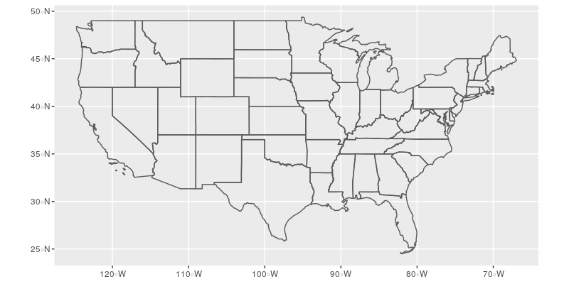
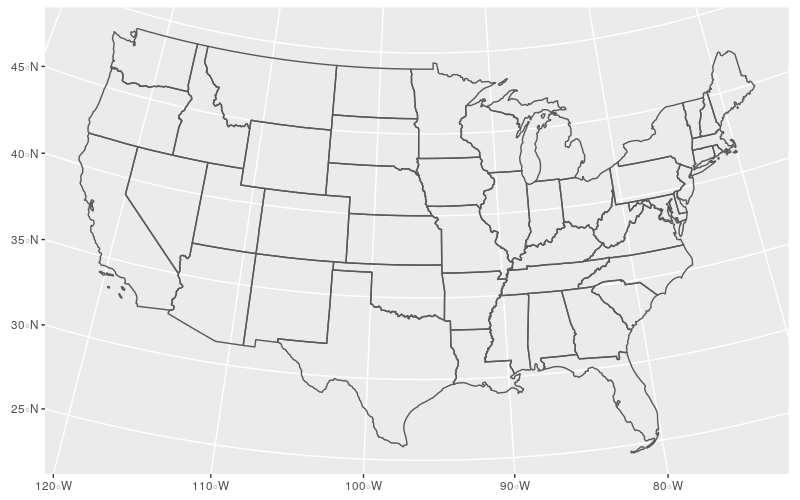
Because an example speaks more than a 1000 of words: consider the USA. The lower 48 are about the right size for a projection to matter. Plus it is an easily recognizable

library(sf)
library(tidyverse)
library(USAboundaries)

usa <- us_boundaries(type="state", resolution = "low") %>% 
  filter(!state_abbr %in% c("PR", "AK", "HI"))  # lower 48 only

wgs84 <- usa %>% 
  st_transform(4326) # WGS84 - good default

albers <- usa %>% 
  st_transform(5070) # Albers - a popular choice for the lower 48

ggplot() +
  geom_sf(data = wgs84, fill = NA)

ggplot() +
  geom_sf(data = albers, fill = NA)

The WGS84 - always a good starting point, but has its shortcomings - draws all parallels as straight lines (watch the Canada border!). This makes the northern states - e.g. Montana - seem bigger than they actually are, compared to those closer to the equator - e.g. Florida. It also looks ugly.

The Albers conical projection is the most common projection for the lower 48. Parallels are not straight (again, watch the Canada border) but the size of the states is more accurate, and the map looks more natural.

To sum my rant up: choosing a "right" projection for your data may be hard, and will depend on your area of interest. Applying it will be easy - with sf::st_transform().

6 Likes

Just to check, could you also do

sessionInfo

I'm on MAC and getting

> library(lwgeom)
Linking to liblwgeom 2.5.0dev r16016, GEOS 3.6.1, PROJ 4.9.3
Warning in fun(libname, pkgname) :
  GEOS versions differ: lwgeom has 3.6.1 sf has 3.7.2
Warning in fun(libname, pkgname) :
  PROJ versions differ: lwgeom has 4.9.3 sf has 5.2.0
> #> Linking to liblwgeom 2.5.0dev r16016, GEOS 3.6.1, PROJ 4.9.3
> #> Warning in fun(libname, pkgname): GEOS versions differ: lwgeom has 3.6.1 sf
> #> has 3.7.2
> #> Warning in fun(libname, pkgname): PROJ versions differ: lwgeom has 4.9.3 sf
> #> has 5.2.0

in addition to your error message. If you're on another OS, I'll switch to my *nix machine.

1 Like

Hi @Dominique, I think @jlacko has the more-than-likely solution, but head back if you get stuck. BTW: Thanks, again, for the reprex!

On second thought: as your data seem to be truly global I suggest you keep the projection as it is.

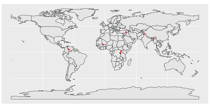
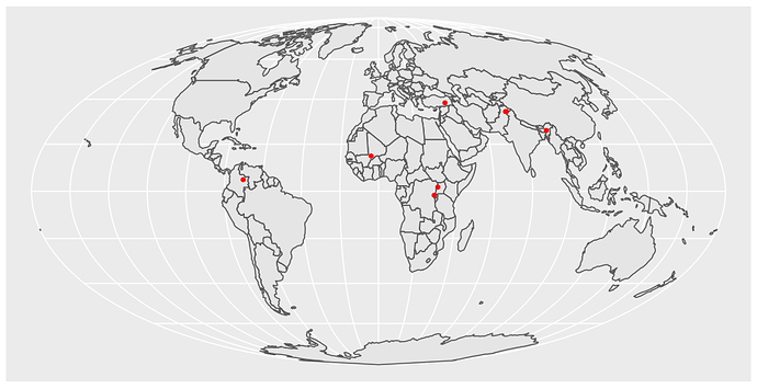
The good ol' Mercator has its well known failings - can you guess the relative size of the United Kingdom and Madagascar just by looking at the map? - but just about everybody is familiar with it.

library(ggplot2)
library(rnaturalearth)

world <- ne_countries(type = 'countries', scale = 'small', returnclass ="sf")

# WGS default
ggplot() +
  geom_sf(data = st_transform(world, 4326)) +
  geom_sf(data = st_transform(conflictMap, 4326), color = "red")

# Mollweide
ggplot() +
  geom_sf(data = st_transform(world, 54009)) +
  geom_sf(data = st_transform(conflictMap, 54009), color = "red")

# Albers
ggplot() +
  geom_sf(data = st_transform(world, 5070)) +
  geom_sf(data = st_transform(conflictMap, 5070), color = "red")

Default = Mercator

Posible alterantive = Mollweide (equal area - see Greenland and Antartica)

Impossible alternative = Albers (good for the USA, but does not make sense for entire world)

1 Like

Hi @jlacko and @technocrat,

Many thanks for your help and explanations - I appreciate it a lot. I have just one follow up question: As I understand now the projection is (at least for what I presented here) mainly for the purpose of visualisation/plotting. Therefore, the projection type has no influence on the accuracy of the mapping (st_join ()). Is that correct?

1 Like

The spatial join - linking points to polygons - will not be affected as long as both objects share CRS (and if I remember correctly the function should fail in case of a CRS mismatch).

On second thought: there may be some funny edge cases when north or south pole is involved - see https://github.com/r-spatial/sf/issues/493 - but yes, in your case the warning can be safely ignored.

2 Likes

Thanks. Luckily, I don't have any points where north or south pole is involved.

Please mark the solution for the benefit of those to follow.

This topic was automatically closed 7 days after the last reply. New replies are no longer allowed.