How to pertubate the fecundity rates of a deterministic matrix model using the popdemo package in R?

[Malaurie]

First of all, I am beginner in R. I am trying to model a population of bullfrogs (deterministic model). I want to evaluate and plot the effects of decreasing the fecundity (of adults) on the population growth rate and survival rates of each life stage. I managed to plot the growth rate of the population but I can't figure out how to properly reduce the fecundity rate using the sensitivity analysis. Not much information can be found on the internet about this subject. I tried the following code (based on the example that can be found in the vignette), but I am not quite sure what number represents the lowering of the fecundity rate. Suppose that I want to lower the fecundity rate by 10%, how should the code look? The matrix looks like this:

|0|0|0|0|0|2082|
|0.369|0|0|0|0|0|
|0|0.232|0|0|0|0|
|0|0|0.207|0|0|0|
|0|0|0|0.047|0|0|
|0|0|0|0|0.042|0.32|

Only the adult fecundity is known (which is 2082). This is the code I tried:

lambda_delta <- numeric(length(delta))
for(i in 1:length(delta)){
  Frog_delta[1, 6] <- data[1, 6] + delta[i]
  lambda_delta[i] <- eigs(Frog_delta, "lambda")
}

[technocrat]

See the FAQ: How to do a minimal reproducible example reprex for beginners. To address the problem as stated, the objects delta and data need to be known, and it's not clear that the matrix

m <- structure(c(0, 0.369, 0, 0, 0, 0, 0, 0, 0.232, 0, 0, 0, 0, 0, 0, 0.207, 0, 0, 0, 0, 0, 0, 0.047, 0, 0, 0, 0, 0, 0, 0.042, 2082, 0, 0, 0, 0, 0.32),
  .Dim =
    c(6L, 6L), .Dimnames = list(NULL, NULL)
)
m
#>       [,1]  [,2]  [,3]  [,4]  [,5]    [,6]
#> [1,] 0.000 0.000 0.000 0.000 0.000 2082.00
#> [2,] 0.369 0.000 0.000 0.000 0.000    0.00
#> [3,] 0.000 0.232 0.000 0.000 0.000    0.00
#> [4,] 0.000 0.000 0.207 0.000 0.000    0.00
#> [5,] 0.000 0.000 0.000 0.047 0.000    0.00
#> [6,] 0.000 0.000 0.000 0.000 0.042    0.32

represents either or something else. And, without a model or algorithm, it is unclear how the matrix is populated from m[1,6], the fecundity.

[Malaurie]

This is the data and the code I tried (copy pasted from the example in the vignette).

data <- data.frame(
   row.names = c("N1", "N2", "N3", "N4", "N5", "N6"),
          N1 = c(0, 0.369, 0, 0, 0, 0),
          N2 = c(0, 0, 0.232, 0, 0, 0),
          N3 = c(0, 0, 0, 0.207, 0, 0),
          N4 = c(0, 0, 0, 0, 0.047, 0),
          N5 = c(0, 0, 0, 0, 0, 0.042),
          N6 = c(2082, 0, 0, 0, 0, 0.32)
)
data2 <- as.matrix(data)
library(popdemo)
delta <- seq(0, 4*data2[1, 6], 0.1)
Frog_delta <- data2
lambda_delta <- numeric(length(delta))
for(i in 1:length(delta)){
  Frog_delta[1, 6] <- data2[1, 6] + delta[i]
  lambda_delta[i] <- eigs(Frog_delta, "lambda")

[technocrat]

The reprex below simplifies the code and explains what it does.

library(popdemo)
#> Welcome to popdemo! This is version 1.3-0
#> Use ?popdemo for an intro, or browseVignettes('popdemo') for vignettes
#> Citation for popdemo is here: doi.org/10.1111/j.2041-210X.2012.00222.x
#> Development and legacy versions are here: github.com/iainmstott/popdemo
                            
dat <- data.frame(
  row.names = c("N1", "N2", "N3", "N4", "N5", "N6"),
  N1 = c(0, 0.369, 0, 0, 0, 0),
  N2 = c(0, 0, 0.232, 0, 0, 0),
  N3 = c(0, 0, 0, 0.207, 0, 0),
  N4 = c(0, 0, 0, 0, 0.047, 0),
  N5 = c(0, 0, 0, 0, 0, 0.042),
  N6 = c(2082, 0, 0, 0, 0, 0.32)
)

delta <- seq(0, 4*dat[1, 6], 0.1)
data_delta <- dat
lambda_delta <- numeric(length(delta))
for(i in 1:length(delta)){
  data_delta[1, 6] <- dat[1, 6] + delta[i]
  lambda_delta[i] <- eigs(data_delta, "lambda")
}

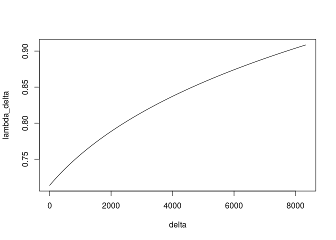
plot(delta, lambda_delta, type = "l")

This reflects the fecundity value at N1,N6 multiplied by 4 and incremented by 0.1 to show and increase of \lambda as the eigenvectors climb.

§6.1 of the vignette shows how to do a sensitivity analysis of the same data

library(popdemo)
#> Welcome to popdemo! This is version 1.3-0
#> Use ?popdemo for an intro, or browseVignettes('popdemo') for vignettes
#> Citation for popdemo is here: doi.org/10.1111/j.2041-210X.2012.00222.x
#> Development and legacy versions are here: github.com/iainmstott/popdemo
                            
dat <- data.frame(
  row.names = c("N1", "N2", "N3", "N4", "N5", "N6"),
  N1 = c(0, 0.369, 0, 0, 0, 0),
  N2 = c(0, 0, 0.232, 0, 0, 0),
  N3 = c(0, 0, 0, 0.207, 0, 0),
  N4 = c(0, 0, 0, 0, 0.047, 0),
  N5 = c(0, 0, 0, 0, 0, 0.042),
  N6 = c(2082, 0, 0, 0, 0, 0.32)
)

tfsm_inertia(as.matrix(dat), bound = "lower", tolerance = 1e-6)
#>           [,1]       [,2]        [,3]       [,4]       [,5]          [,6]
#> [1,] 0.0000000 0.00000000  0.00000000  0.0000000  0.0000000 -6.573952e-06
#> [2,] 0.2560898 0.00000000  0.00000000  0.0000000  0.0000000  0.000000e+00
#> [3,] 0.0000000 0.08016566  0.00000000  0.0000000  0.0000000  0.000000e+00
#> [4,] 0.0000000 0.00000000 -0.02935737  0.0000000  0.0000000  0.000000e+00
#> [5,] 0.0000000 0.00000000  0.00000000 -0.2815965  0.0000000  0.000000e+00
#> [6,] 0.0000000 0.00000000  0.00000000  0.0000000 -0.3263449 -2.072519e-01