How to move geom_polygon ?

Andrzej · November 23, 2024, 8:09am

I have this data:

dat <- structure(list(ID = c(1, 1, 2, 2, 3, 3, 4, 4, 5, 5, 6, 6, 7, 
7, 8, 8, 9, 9, 10, 10, 11, 11, 12, 12, 13, 13, 14, 14, 15, 15, 
16, 16, 17, 17, 18, 18, 19, 19, 20, 20, 21, 21, 22, 22, 23, 23, 
24, 24, 25, 25, 26, 26, 27, 27, 28, 28, 29, 29, 30, 30, 31, 31, 
32, 32, 33, 33, 34, 34, 35, 35, 36, 36, 37, 37, 38, 38, 39, 39, 
40, 40, 41, 41, 42, 42, 43, 43, 44, 44, 45, 45, 46, 46, 47, 47, 
48, 48, 49, 49, 50, 50, 51, 51, 52, 52, 53, 53, 54, 54, 55, 55, 
56, 56, 57, 57, 58, 58, 59, 59, 60, 60, 61, 61, 62, 62, 63, 63, 
64, 64, 65, 65, 66, 66, 67, 67, 68, 68, 69, 69, 70, 70, 71, 71, 
72, 72, 73, 73, 74, 74, 75, 75, 76, 76, 77, 77, 78, 78, 79, 79, 
80, 80, 81, 81, 82, 82, 83, 83, 84, 84, 85, 85, 86, 86, 87, 87, 
88, 88, 89, 89, 90, 90, 91, 91, 92, 92, 93, 93, 94, 94, 95, 95, 
96, 96, 97, 97, 98, 98, 99, 99, 100, 100, 101, 101, 102, 102, 
103, 103, 104, 104, 105, 105, 106, 106, 107, 107, 108, 108, 109, 
109, 110, 110, 111, 111, 112, 112, 113, 113, 114, 114, 115, 115, 
116, 116, 117, 117, 118, 118, 119, 119, 120, 120, 121, 121, 122, 
122, 123, 123, 124, 124, 125, 125, 126, 126, 127, 127, 128, 128
), Examination = c(1, 2, 1, 2, 1, 2, 1, 2, 1, 2, 1, 2, 1, 2, 
1, 2, 1, 2, 1, 2, 1, 2, 1, 2, 1, 2, 1, 2, 1, 2, 1, 2, 1, 2, 1, 
2, 1, 2, 1, 2, 1, 2, 1, 2, 1, 2, 1, 2, 1, 2, 1, 2, 1, 2, 1, 2, 
1, 2, 1, 2, 1, 2, 1, 2, 1, 2, 1, 2, 1, 2, 1, 2, 1, 2, 1, 2, 1, 
2, 1, 2, 1, 2, 1, 2, 1, 2, 1, 2, 1, 2, 1, 2, 1, 2, 1, 2, 1, 2, 
1, 2, 1, 2, 1, 2, 1, 2, 1, 2, 1, 2, 1, 2, 1, 2, 1, 2, 1, 2, 1, 
2, 1, 2, 1, 2, 1, 2, 1, 2, 1, 2, 1, 2, 1, 2, 1, 2, 1, 2, 1, 2, 
1, 2, 1, 2, 1, 2, 1, 2, 1, 2, 1, 2, 1, 2, 1, 2, 1, 2, 1, 2, 1, 
2, 1, 2, 1, 2, 1, 2, 1, 2, 1, 2, 1, 2, 1, 2, 1, 2, 1, 2, 1, 2, 
1, 2, 1, 2, 1, 2, 1, 2, 1, 2, 1, 2, 1, 2, 1, 2, 1, 2, 1, 2, 1, 
2, 1, 2, 1, 2, 1, 2, 1, 2, 1, 2, 1, 2, 1, 2, 1, 2, 1, 2, 1, 2, 
1, 2, 1, 2, 1, 2, 1, 2, 1, 2, 1, 2, 1, 2, 1, 2, 1, 2, 1, 2, 1, 
2, 1, 2, 1, 2, 1, 2, 1, 2, 1, 2), Opening = c(31, 41, 29, 
43, 34, 47, 28, 42, 29, 44, 31, 41, 33, 43, 29, 42, 28, 42, 29, 
43, 28, 43, 28, 45, 31, 41, 30, 43, 31, 41, 32, 44, 31, 46, 28, 
45, 29, 44, 31, 45, 33, 44, 34, 47, 31, 41, 31, 43, 32, 45, 34, 
45, 32, 41, 29, 42, 28, 43, 31, 41, 31, 41, 33, 46, 32, 47, 34, 
43, 33, 45, 34, 43, 34, 45, 34, 45, 32, 43, 32, 42, 31, 45, 29, 
46, 28, 49, 31, 46, 33, 43, 31, 45, 32, 41, 32, 43, 32, 45, 34, 
41, 31, 45, 31, 41, 32, 45, 32, 46, 28, 45, 28, 43, 27, 41, 31, 
41, 34, 43, 31, 48, 31, 49, 32, 51, 34, 45, 31, 41, 32, 46, 33, 
45, 32, 41, 33, 43, 33, 41, 31, 45, 29, 46, 31, 41, 32, 43, 31, 
45, 32, 45, 31, 46, 32, 41, 30, 46, 31, 48, 31, 45, 32, 46, 30, 
42, 34, 43, 32, 42, 34, 43, 34, 44, 31, 41, 32, 44, 32, 47, 33, 
41, 31, 49, 29, 43, 34, 44, 31, 42, 32, 41, 35, 41, 32, 41, 34, 
45, 32, 46, 34, 46, 33, 48, 33, 47, 31, 43, 33, 44, 32, 45, 33, 
41, 31, 44, 32, 43, 32, 45, 32, 47, 34, 44, 34, 41, 32, 46, 28, 
46, 31, 45, 29, 46, 34, 45, 34, 41, 33, 42, 34, 41, 31, 41, 33, 
42, 32, 41, 31, 43, 31, 43, 32, 41, 29, 41, 34, 45)), class = "data.frame", row.names = c(NA, 
-256L), variable.labels = structure(character(0), names = character(0)), codepage = 65001L)

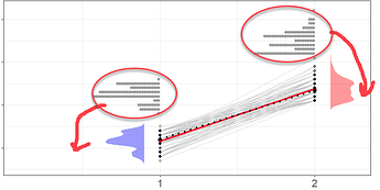
and I want to get this plot:
https://stackoverflow.com/questions/56588746/combine-spaghetti-plot-with-a-grouping-variable-with-split-violins-without-it

I have tried this:

density_data <- dat %>%
  group_by(Examination) %>%
  do({
    dens <- density(.$Opening)
    data.frame(
      loc = dens$x,
      dens = dens$y,
      Examination = unique(.$Examination)
    )
  }) %>%
  mutate(dens = ifelse(Examination == 1, -dens, dens))

plot <- ggplot(dat, aes(x = factor(Examination), y = Opening)) +
  geom_point(size = 3, alpha = 0.6) +
  geom_line(aes(group = ID), size = 1, alpha = 0.5) +
  xlab("Examination") +
  ylab("Opening") +
  theme_minimal() +
  geom_polygon(
    data = density_data,
    aes(x = dens, y = loc, fill = factor(Examination), group = Examination),
    alpha = 0.4
  ) +
  scale_fill_manual(values = c("1" = "blue", "2" = "red")) +
  theme(legend.position = "top")

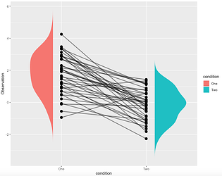
but it gives me this:

I want to move upper geom_polygon to the right hand side of the plot where the data for it are placed like in previous plot from SO solution. Any help much appreciated, thank you.

FJCC · November 23, 2024, 1:36pm

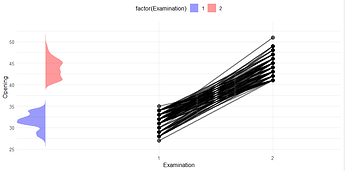
I adjusted the density values by the desired shift.

library(tidyverse)
dat <- structure(list(ID = c(1, 1, 2, 2, 3, 3, 4, 4, 5, 5, 6, 6, 7, 
7, 8, 8, 9, 9, 10, 10, 11, 11, 12, 12, 13, 13, 14, 14, 15, 15, 
16, 16, 17, 17, 18, 18, 19, 19, 20, 20, 21, 21, 22, 22, 23, 23, 
24, 24, 25, 25, 26, 26, 27, 27, 28, 28, 29, 29, 30, 30, 31, 31, 
32, 32, 33, 33, 34, 34, 35, 35, 36, 36, 37, 37, 38, 38, 39, 39, 
40, 40, 41, 41, 42, 42, 43, 43, 44, 44, 45, 45, 46, 46, 47, 47, 
48, 48, 49, 49, 50, 50, 51, 51, 52, 52, 53, 53, 54, 54, 55, 55, 
56, 56, 57, 57, 58, 58, 59, 59, 60, 60, 61, 61, 62, 62, 63, 63, 
64, 64, 65, 65, 66, 66, 67, 67, 68, 68, 69, 69, 70, 70, 71, 71, 
72, 72, 73, 73, 74, 74, 75, 75, 76, 76, 77, 77, 78, 78, 79, 79, 
80, 80, 81, 81, 82, 82, 83, 83, 84, 84, 85, 85, 86, 86, 87, 87, 
88, 88, 89, 89, 90, 90, 91, 91, 92, 92, 93, 93, 94, 94, 95, 95, 
96, 96, 97, 97, 98, 98, 99, 99, 100, 100, 101, 101, 102, 102, 
103, 103, 104, 104, 105, 105, 106, 106, 107, 107, 108, 108, 109, 
109, 110, 110, 111, 111, 112, 112, 113, 113, 114, 114, 115, 115, 
116, 116, 117, 117, 118, 118, 119, 119, 120, 120, 121, 121, 122, 
122, 123, 123, 124, 124, 125, 125, 126, 126, 127, 127, 128, 128
), Examination = c(1, 2, 1, 2, 1, 2, 1, 2, 1, 2, 1, 2, 1, 2, 
1, 2, 1, 2, 1, 2, 1, 2, 1, 2, 1, 2, 1, 2, 1, 2, 1, 2, 1, 2, 1, 
2, 1, 2, 1, 2, 1, 2, 1, 2, 1, 2, 1, 2, 1, 2, 1, 2, 1, 2, 1, 2, 
1, 2, 1, 2, 1, 2, 1, 2, 1, 2, 1, 2, 1, 2, 1, 2, 1, 2, 1, 2, 1, 
2, 1, 2, 1, 2, 1, 2, 1, 2, 1, 2, 1, 2, 1, 2, 1, 2, 1, 2, 1, 2, 
1, 2, 1, 2, 1, 2, 1, 2, 1, 2, 1, 2, 1, 2, 1, 2, 1, 2, 1, 2, 1, 
2, 1, 2, 1, 2, 1, 2, 1, 2, 1, 2, 1, 2, 1, 2, 1, 2, 1, 2, 1, 2, 
1, 2, 1, 2, 1, 2, 1, 2, 1, 2, 1, 2, 1, 2, 1, 2, 1, 2, 1, 2, 1, 
2, 1, 2, 1, 2, 1, 2, 1, 2, 1, 2, 1, 2, 1, 2, 1, 2, 1, 2, 1, 2, 
1, 2, 1, 2, 1, 2, 1, 2, 1, 2, 1, 2, 1, 2, 1, 2, 1, 2, 1, 2, 1, 
2, 1, 2, 1, 2, 1, 2, 1, 2, 1, 2, 1, 2, 1, 2, 1, 2, 1, 2, 1, 2, 
1, 2, 1, 2, 1, 2, 1, 2, 1, 2, 1, 2, 1, 2, 1, 2, 1, 2, 1, 2, 1, 
2, 1, 2, 1, 2, 1, 2, 1, 2, 1, 2), Opening = c(31, 41, 29, 
43, 34, 47, 28, 42, 29, 44, 31, 41, 33, 43, 29, 42, 28, 42, 29, 
43, 28, 43, 28, 45, 31, 41, 30, 43, 31, 41, 32, 44, 31, 46, 28, 
45, 29, 44, 31, 45, 33, 44, 34, 47, 31, 41, 31, 43, 32, 45, 34, 
45, 32, 41, 29, 42, 28, 43, 31, 41, 31, 41, 33, 46, 32, 47, 34, 
43, 33, 45, 34, 43, 34, 45, 34, 45, 32, 43, 32, 42, 31, 45, 29, 
46, 28, 49, 31, 46, 33, 43, 31, 45, 32, 41, 32, 43, 32, 45, 34, 
41, 31, 45, 31, 41, 32, 45, 32, 46, 28, 45, 28, 43, 27, 41, 31, 
41, 34, 43, 31, 48, 31, 49, 32, 51, 34, 45, 31, 41, 32, 46, 33, 
45, 32, 41, 33, 43, 33, 41, 31, 45, 29, 46, 31, 41, 32, 43, 31, 
45, 32, 45, 31, 46, 32, 41, 30, 46, 31, 48, 31, 45, 32, 46, 30, 
42, 34, 43, 32, 42, 34, 43, 34, 44, 31, 41, 32, 44, 32, 47, 33, 
41, 31, 49, 29, 43, 34, 44, 31, 42, 32, 41, 35, 41, 32, 41, 34, 
45, 32, 46, 34, 46, 33, 48, 33, 47, 31, 43, 33, 44, 32, 45, 33, 
41, 31, 44, 32, 43, 32, 45, 32, 47, 34, 44, 34, 41, 32, 46, 28, 
46, 31, 45, 29, 46, 34, 45, 34, 41, 33, 42, 34, 41, 31, 41, 33, 
42, 32, 41, 31, 43, 31, 43, 32, 41, 29, 41, 34, 45)), class = "data.frame", row.names = c(NA, 
-256L), variable.labels = structure(character(0), names = character(0)), codepage = 65001L)

density_data <- dat %>%
  group_by(Examination) %>%
  do({
    dens <- density(.$Opening)
    data.frame(
      loc = dens$x,
      dens = dens$y,
      Examination = unique(.$Examination)
    )
  }) %>%
  mutate(dens = ifelse(Examination == 1, 0.9 - dens, 2.1 + dens))

plot <- ggplot(dat, aes(x = factor(Examination), y = Opening)) +
  geom_point(size = 3, alpha = 0.6) +
  geom_line(aes(group = ID), size = 1, alpha = 0.5) +
  xlab("Examination") +
  ylab("Opening") +
  theme_minimal() +
  geom_polygon(
    data = density_data,
    aes(x = dens, y = loc, fill = factor(Examination), group = Examination),
    alpha = 0.4
  ) +
  scale_fill_manual(values = c("1" = "blue", "2" = "red")) +
  theme(legend.position = "top")
#> Warning: Using `size` aesthetic for lines was deprecated in ggplot2 3.4.0.
#> ℹ Please use `linewidth` instead.
#> This warning is displayed once every 8 hours.
#> Call `lifecycle::last_lifecycle_warnings()` to see where this warning was
#> generated.
plot

^{Created on 2024-11-23 with reprex v2.1.1}

Andrzej · November 23, 2024, 1:43pm

Thank you, can you please explain what does that line above do ?

Where did 0.9 and 2.1 come from ?

FJCC · November 23, 2024, 2:24pm

The levels of a factor have the numeric values 1, 2, 3, ... I can place the base of the density distributions on top of the data points by using

mutate(dens = ifelse(Examination == 1,  1 - dens, 2 + dens))

In your original plot, you effectively had

mutate(dens = ifelse(Examination == 1,  0 - dens, 0 + dens))

so your density distributions were to the left of all the data points.

I chose 0.9 and 2.1 to shift the density distributions away from the data points but have each distribution near its corresponding data points

Andrzej · November 23, 2024, 3:53pm

Thank you, very informative.

Andrzej · November 24, 2024, 1:10pm

I want to tweak this plot further,
how to add geom_half_boxplot, geom_pointrange(aes(y = Mean, ymin = Mean - SD, ymax = Mean+SD) and
geom_dotplot() to it ?
Is it possible to separate dot plots and move them separately ?

system · December 1, 2024, 1:11pm

This topic was automatically closed 7 days after the last reply. New replies are no longer allowed.

If you have a query related to it or one of the replies, start a new topic and refer back with a link.