How to make stat_summary of each group?

Hello everyone! I have a dataset with Metabolite concentration (triplicate measurement) with 2 Types (Product1, 2), in Time series (0,2,4 weeks) and in different Temperatures (0,25,40,FT). I'd like to plot mean and SD for each Product at each Timepoint and each Temperature with stat_summary.

However, stat_summary cannot identify colour as a variable - and pools all points from Type, hereby calculating/plotting the average and SD of all Products pooled. What I'd like to do is rather make mean+SD for each individual Product in different temperatures per Timepoint in dedicated colors.

How could it be done? Thank you :slight_smile:

summary(dataLPstability)
dataLPstability$Type <- factor(dataLPstability$Type, levels = c('Product1,'Product2'), ordered = TRUE) #converting Formulation to factorial
dataLPstability$Temperature <- factor(dataLPstability$Temperature, levels = c('0','25','40','FT'), ordered = TRUE)

##Plotting
line.MetaboliteA <- ggplot(dataLPstability, mapping = aes(x=Time,y=MetaboliteA,color=Temperature, group=Type))+geom_point() + stat_summary(fun = "mean", geom= "line",size=1) + facet_grid(vars(Type),vars(Temperature), scales = "free")+ labs(x="Week", y="Concentration, mg/L", title="Metabolite A")

line.MetaboliteA + scale_x_continuous(breaks = scales::pretty_breaks(n = 6)) + theme_base()+ stat_summary(fun.data = "mean_sdl", fun.args=list(mult=2), geom= "linerange",color="blue",size=0.5)
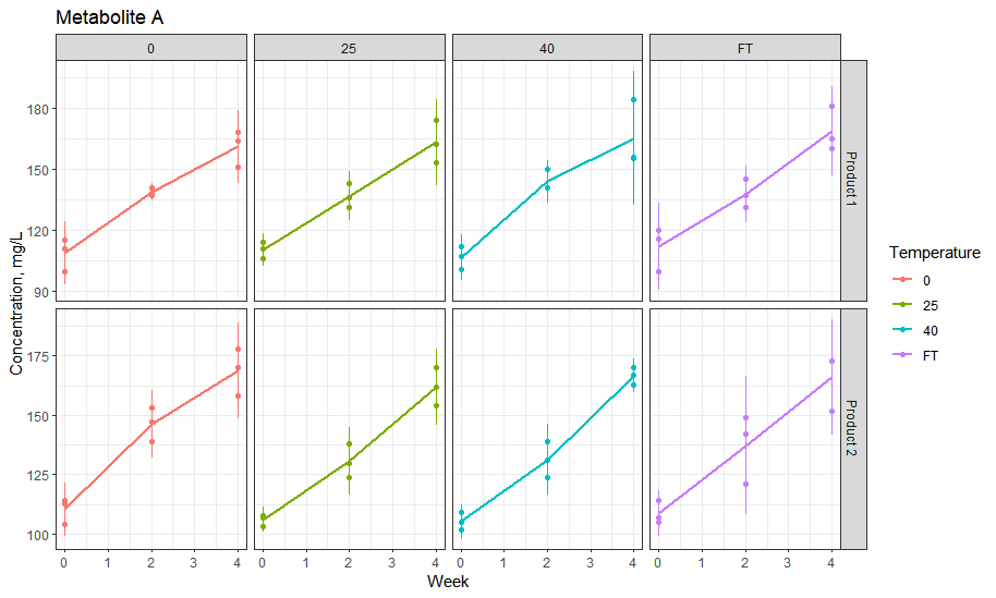
# Add colors column to mtcars dataset
# get some colors
paint <- sample(colors(),8)
mtcars$colors <- as.factor(sample(paint,32,replace = TRUE))
# Use aggregate() function to get summary statistics by colors
summary_by_colors <- aggregate(. ~ colors, data = mtcars, FUN = summary)
summary_by_colors[,1:4]
#>       colors mpg.Min. mpg.1st Qu. mpg.Median mpg.Mean mpg.3rd Qu. mpg.Max.
#> 1      beige 15.00000    19.50000   21.00000 20.35000    21.85000 24.40000
#> 2    bisque1 10.40000    18.50000   21.50000 21.62857    25.05000 32.40000
#> 3  cornsilk1 14.30000    23.07500   28.20000 26.15000    31.27500 33.90000
#> 4 goldenrod2 10.40000    16.40000   21.40000 20.28000    22.80000 30.40000
#> 5 goldenrod3 13.30000    14.65000   16.00000 16.00000    17.35000 18.70000
#> 6     gray16 15.20000    15.35000   15.50000 16.63333    17.35000 19.20000
#> 7      gray5 14.70000    15.52500   16.55000 16.47500    17.50000 18.10000
#> 8     grey32 15.20000    17.45000   19.70000 18.76667    20.55000 21.40000
#>   cyl.Min. cyl.1st Qu. cyl.Median cyl.Mean cyl.3rd Qu. cyl.Max. disp.Min.
#> 1 4.000000    5.500000   6.000000 6.000000    6.500000 8.000000  146.7000
#> 2 4.000000    4.000000   4.000000 5.428571    7.000000 8.000000   78.7000
#> 3 4.000000    4.000000   4.000000 5.000000    5.000000 8.000000   71.1000
#> 4 4.000000    4.000000   4.000000 5.600000    8.000000 8.000000   95.1000
#> 5 8.000000    8.000000   8.000000 8.000000    8.000000 8.000000  350.0000
#> 6 6.000000    7.000000   8.000000 7.333333    8.000000 8.000000  167.6000
#> 7 6.000000    7.500000   8.000000 7.500000    8.000000 8.000000  225.0000
#> 8 6.000000    6.000000   6.000000 6.666667    7.000000 8.000000  145.0000
#>   disp.1st Qu. disp.Median disp.Mean disp.3rd Qu. disp.Max.
#> 1     156.6750    160.0000  191.9250     195.2500  301.0000
#> 2      93.5000    120.1000  201.9143     283.8000  460.0000
#> 3      74.5500     98.0000  156.7750     180.2250  360.0000
#> 4     121.0000    140.8000  220.9400     275.8000  472.0000
#> 5     352.5000    355.0000  355.0000     357.5000  360.0000
#> 6     235.8000    304.0000  263.2000     311.0000  318.0000
#> 7     263.1000    313.4000  322.9500     373.2500  440.0000
#> 8     201.5000    258.0000  226.2667     266.9000  275.8000

Created on 2023-09-06 with reprex v2.0.2

Like this?

dataLPstability = 
structure(list(Type = c("Product 1", "Product 1", "Product 1", 
"Product 1", "Product 1", "Product 1", "Product 1", "Product 1", 
"Product 1", "Product 1", "Product 1", "Product 2", "Product 2", 
"Product 2", "Product 2", "Product 2", "Product 2", "Product 2", 
"Product 2", "Product 2", "Product 2", "Product 2"), Temperature = c("0", 
"0", "0", "0", "0", "0", "0", "0", "0", "25", "25", "25", "25", 
"25", "25", "25", "25", "25", "40", "40", "40", "40", "40", "40", 
"40", "40", "40", "FT", "FT", "FT", "FT", "FT", "FT", "FT", "FT", 
"FT", "0", "0", "0", "0", "0", "0", "0", "0", "0", "25", "25", 
"25", "25", "25", "25", "25", "25", "25", "40", "40", "40", "40", 
"40", "40", "40", "40", "40", "FT", "FT", "FT", "FT", "FT", "FT", 
"FT", "FT", "FT"), Time = c(0, 0, 0, 2, 2, 2, 4, 4, 4, 0, 0, 
0, 2, 2, 2, 4, 4, 4, 0, 0, 0, 2, 2, 2, 4, 4, 4, 0, 0, 0, 2, 2, 
2, 4, 4, 4, 0, 0, 0, 2, 2, 2, 4, 4, 4, 0, 0, 0, 2, 2, 2, 4, 4, 
4, 0, 0, 0, 2, 2, 2, 4, 4, 4, 0, 0, 0, 2, 2, 2, 4, 4, 4), Rep = c(1, 
2, 3, 1, 2, 3, 1, 2, 3, 1, 2, 3, 1, 2, 3, 1, 2, 3, 1, 2, 3, 1, 
2, 3, 1, 2, 3, 1, 2, 3, 1, 2, 3, 1, 2, 3, 1, 2, 3, 1, 2, 3, 1, 
2, 3, 1, 2, 3, 1, 2, 3, 1, 2, 3, 1, 2, 3, 1, 2, 3, 1, 2, 3, 1, 
2, 3, 1, 2, 3, 1, 2, 3), MetaboliteA = c(115, 100, 111, 138, 
137, 141, 151, 168, 164, 106, 114, 111, 131, 143, 136, 153, 162, 
174, 101, 112, 107, 141, 141, 150, 156, 155, 184, 120, 100, 116, 
137, 145, 131, 165, 160, 181, 104, 113, 114, 153, 147, 139, 178, 
158, 170, 108, 103, 107, 130, 138, 124, 162, 154, 170, 102, 105, 
109, 124, 131, 139, 163, 167, 170, 114, 105, 107, 121, 142, 149, 
173, 152, 173)), class = c("tbl_df", "tbl", "data.frame"), row.names = c(NA, 
-72L))

ggplot(dataLPstability, 
       mapping = aes(x=Time, 
                     y=MetaboliteA,
                     color=Temperature)) +
   geom_point() + 
   stat_summary(fun = "mean", geom= "line",size=1) + 
   facet_grid(vars(Type),vars(Temperature), scales = "free") + 
   labs(x="Week", y="Concentration, mg/L", title="Metabolite A") +
   stat_summary(fun.data = "mean_sdl", fun.args=list(mult=2), 
                geom= "linerange", size=0.5,
                show.legend = FALSE) +
   theme_bw()

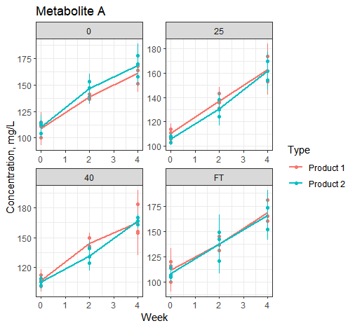
Somewhat, but having Product 1 and 2 on the same graphs (i.e. one row in the facet grid). This graph I could do myself, but when Products become on top of each other, this is where the fun starts.

This wasn't part of your example.
Like this?

ggplot(dataLPstability, 
       mapping = aes(x=Time, y=MetaboliteA,
                     color=Type)) +
   geom_point() + 
   stat_summary(fun = "mean", geom= "line",size=1) + 
   facet_wrap(vars(Temperature), scales = "free") + 
   labs(x="Week", y="Concentration, mg/L", title="Metabolite A") +
   stat_summary(fun.data = "mean_sdl", fun.args=list(mult=2), 
                geom= "linerange", size=0.5,
                show.legend = FALSE) +
   theme_bw()

grafik

Yes! :slight_smile: Indeed, that is the way, I'd like!

This topic was automatically closed 21 days after the last reply. New replies are no longer allowed.

If you have a query related to it or one of the replies, start a new topic and refer back with a link.