An example with two of your data frames. It might be a bit of repetitive work though. If you want to automate, you could read several files in one go but that's more advanced. For an example see here and here.
library(tidyverse)
#Data for D1
d1 <- structure(list(Time = c(3.891667, 3.9, 3.908333, 3.916667, 3.925, 3.933333, 3.941667, 3.95, 3.958333, 3.966667), PRN = c(1, 1, 1, 1, 1, 1, 1, 1, 1, 1), Lat = c(-10.728, -10.649, -10.571, -10.494, -10.417, -10.341, -10.266, -10.192, -10.119, -10.046), Lon = c(141.988, 142.036, 142.084, 142.131, 142.177, 142.223, 142.268, 142.313, 142.357, 142.4), Stec = c(33.99, 34.41, 34.58, 35.01, 35.18, 35.44, 35.52, 35.58, 35.41, 35.54)), row.names = c(NA, -10L), class = c("tbl_df", "tbl", "data.frame"))
#Data for D2
d2 <- structure(list(Time = c(3.783333, 3.791667, 3.8, 3.808333, 3.816667, 3.825, 3.858333, 3.866667, 3.875, 3.883333), PRN = c(1, 1, 1, 1, 1, 1, 1, 1, 1, 1), Lat = c(-11.116, -11.033, -10.951, -10.87, -10.789, -10.71, -10.399, -10.324, -10.249, -10.175), Lon = c(141.746, 141.798, 141.849, 141.899, 141.949, 141.998, 142.187, 142.233, 142.278, 142.322), Stec = c(19.93, 20.03, 20.3, 20.32, 20.2, 20.59, 20.59, 20.74, 20.8, 20.72)), row.names = c(NA, -10L), class = c("tbl_df", "tbl", "data.frame"))
df1 <-
d1 %>%
mutate(id = "30-4-19") %>%
bind_rows(d2 %>% mutate(id = "1-5-19")) %>%
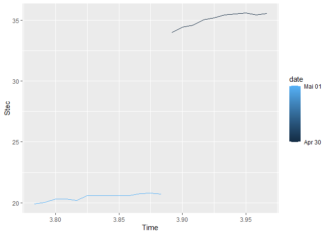
mutate(date = lubridate::dmy(id))
ggplot(df1, aes(x = Time, y = Stec))+
geom_line(aes(color = date, group = date))
df2 <-
d1 %>%
mutate(id = "30-4-19") %>%
bind_rows(d2 %>% mutate(id = "1-5-19")) %>%
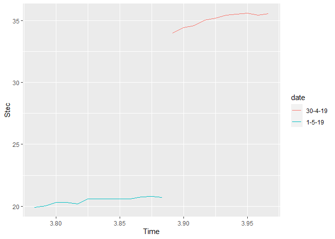
mutate(date = factor(id, levels = c("30-4-19", "1-5-19")))
ggplot(df2, aes(x = Time, y = Stec))+
geom_line(aes(color = date, group = date))
Created on 2020-07-06 by the reprex package (v0.3.0)