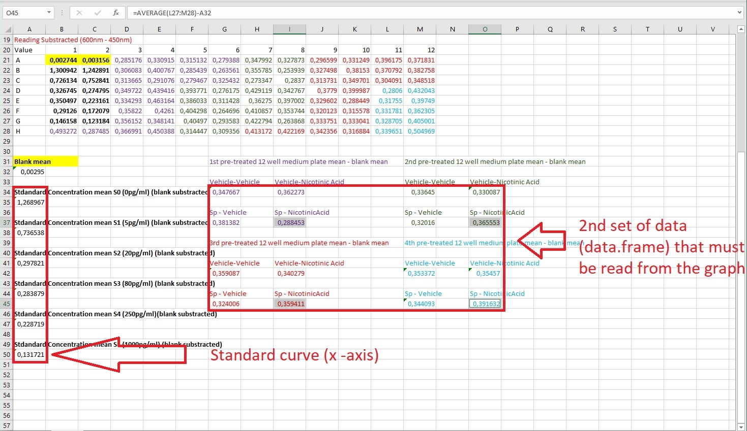
Hello everyone,
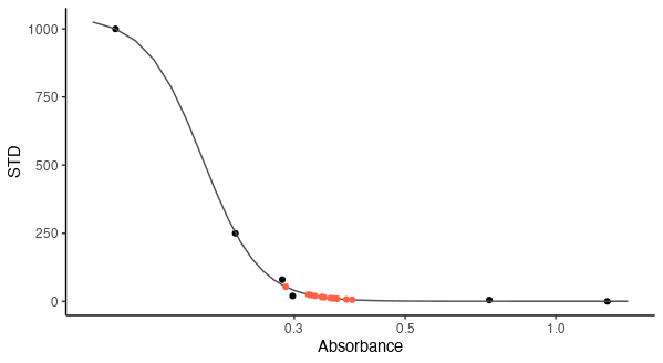
I have recently been working on producing a standard curve with a non-linear regression line that would be presented with a 4 parameter logistic function. I managed to achieve that by using the dcr and plotrix packages, and I got
by using the following code:
library(drc)
library(plotrix)
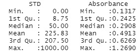
x <- c(0, 1.2689671, 0.7365379, 0.2978207, 0.2838790, 0.2287194, 0.1317211)
y <- c(0, 5, 20, 80, 250, 1000)
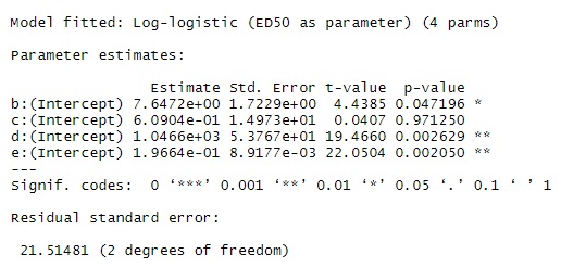
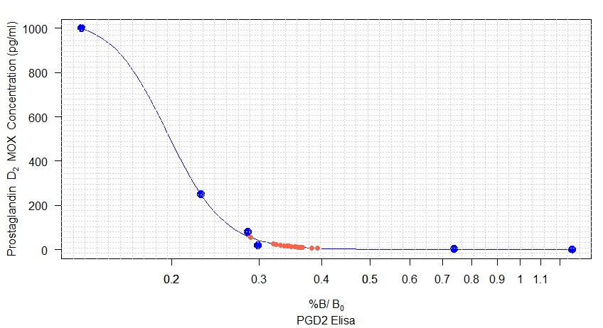
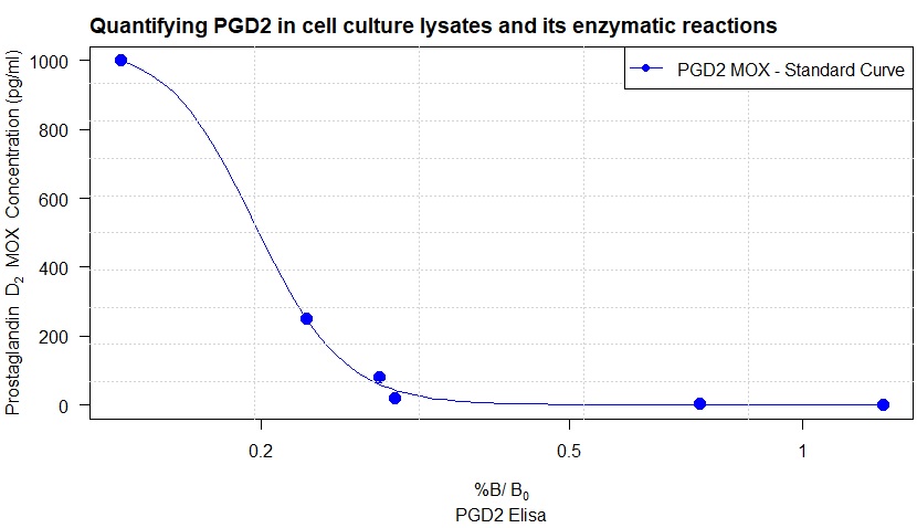
model <- drm(STD ~ Absorbance, fct = LL.4(), data = STD)
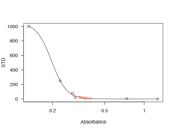
plot(model, cex=1.5,
col= "blue",
pch=16,
sub = "PGD2 Elisa",
xlab = expression(paste("%B/"~B[0]),size = 1, adj= 0),
ylab = expression(paste("Prostaglandin" ~~~ D[2], ~~"MOX Concentration (pg/ml) "))
)+
title("Quantifying PGD2 in cell culture lysates and its enzymatic reactions ", adj = 0)+
grid(5,10)+
legend("topright", legend = c("PGD2 MOX - Standard Curve"),
lwd = 1.5, pch=16, col = c("blue")
)
However, the graph above is the visual representation of the biosynthetic assay. After fitting the line by non-linear regression, now I have to convert the sample absorbance (the second set of data) to pg/ml PGD2 (y-axis). I could do it manually, but first of all, it would not be precise, it is time-consuming, and by using Rstudio, I can improve my coding knowledge. Therefore, I have been thinking of data.frame that I was using while working with ggplot2 , so I created the following data.frame :
DataFramePGD2<-structure(list(Drug = structure(c(1L, 1L, 1L, 1L, 5L, 5L, 5L, 5L, 4L, 4L, 4L, 4L, 3L, 3L, 3L, 3L, 2L, 2L, 2L, 2L),
                                               .Label = c("Vehicle-Vehicle", "Vehicle-NicAcid", "SP-Vehicle", "SP-NicAcid"),
                                                class = "factor"), Absorbance = c(0.3476667, 0.3364504, 0.3590866, 0.3533717,
                                                                                  0.3622728, 0.3300868, 0.3402785, 0.3545702,
                                                                                  0.3813823, 0.3201596, 0.3240057, 0.3440934,
                                                                                  0.2884533, 0.3655528, 0.3594112, 0.3916317)), class = "data.frame", row.names = c(NA,
                                                                                                                                                                      -16L))
However, I never used data.frame within basic r graphics, and I do not know how to make my data.frame be fitted within the graph. I do not know what kind of code to use and how to do it.
DataUsed to produce above graph
DataUsed to produce data.frame
Thank you for any help