How to find the corresponding grid centroids

I have two dataframes, and they both have lat (represents latitude) and lon (represents longitude). The dataframe "obst" contains the coordinates of observation stations, while the dataframe "pr_df" contains the coordinates (as gridded data) and precipitation values in the whole region of the study. The coordinates of "obst" may be within a grid cell, or on the edge of a grid cell. Now for each coordinate pair (which represents an observation station) in the "obst" dataframe, I want to find the corresponding grid cell in the "pr_df" dataframe. How to do this?
I give a small sample and the overlay code that I have. Thanks for your help.

obst # open the obs stations and overlay on the map
lat lon
36 106.5
37 107
37.6 106

pr_df
lat lon pr
35 106 1.5
35 106.5 2
35 107 1.8
35 107.5 2.2
35 108 3.0
35.5 106 1.6
...
35 108 3.4

surface.all= ggplot()+ my_year+ my_fill+ geom_tile(data=pr_df,aes(y=lat,x=lon,fill=pr)) +
coord_quickmap(xlim=range(pr_df$lon), ylim=range(pr_df$lat))+
borders('world', xlim=range(pr_df$lon), ylim=range(pr_df$lat), colour='black')+
geom_point(data=obst,aes(y=lat,x=lon),colour='dark green')+
guides(fill=guide_legend(title="Precipitation"))
print(surface.all) # overlay the stations

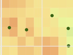
The resulting figure is like this figure, but since my grid cells are small and very organized squares, a grid cell can only contain one observation station. Also, there are many grid cells, but just a small number of observation stations. Thanks for your help.

Actually, I just checked that there can be two stations in one grid cell. In most cases, one grid cell contains just one station, if not intersect with the station location.
Thanks for any help..

I would suggest looking at the sf package if you haven’t already done so. You can project both of your data frames as sf objects and use st_intersection() to combine the two geometries. I would place your point data in the x argument, and would also subset the columns of your grid data into a new object that contains just the ID variable and the geometry of the grid squares. Use that subset version of your grid as the y argument data for the intersection.

Thanks, but I could not find an example about converting data frames to sf objects.
I can write consecutive numbers as the ID variable, but what about geometry? I think the grid squares all have the same lengths. Thanks again.

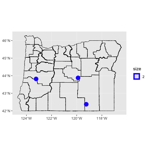
hey @Ellenz - I can try to help with this. I've made a really simple reproducible example of your sample data above. This shows you how to project your latitude/longitude based data as an sf object and overlays them on a county shapefiles of Oregon, as you had above.

library(ggplot2)  # plot data
library(sf)       # spatial tools
library(tigris)   # download tiger/line data

# create sample data
data <- data.frame(
  id = c(1, 2, 3),
  x = c(-119.240707, -119.893685, -123.228394),
  y = c(42.373192, 43.876890, 43.815685)
)

# transfer to sf object
data_sf <- st_as_sf(data, coords = c("x", "y"), crs = 4269)

# download county data
counties <- counties(state = "OR", class = "sf")

# plot sample data
ggplot() +
  geom_sf(data = counties, fill = NA, color = "#000000", size = .25) +
  geom_sf(data_sf, mapping = aes(size = 2), color = "#2200ff")

oregon

What I can't help you with based on the original post is how to get your grid squares into an sf object. Can you tell me how you created the tessellation? Was it made using ArcGIS or QGIS? What file format is it currently saved in?

1 Like

Thanks. The grid squares are from the netcdf files initially, so that the latitude and longitude are fixed. I then just converted them to a dataframe with three columns: latitude, longitude, and precipitation.

Gotcha. I’m not a user of netCDF data so my advice is limited. You may be able read it in with st_read() if it contains vector data. I also found this resource from the University of Oregon that looks promising if your file contains raster data.

I think the problem is not with netcdf data, as I have already read the data. I was thinking if it is possible to work with sf from the dataframes. Also, when downloading county data, is this limited to the U.S. only? If I want to download data from other countries, how to do that? Thanks for your help.

From what I read, the key is to read the netCDF data in in a way that the geometry is preserved. It sounds like these grided data are usually rasters? Instead of converting them to data frames, converting them to vectors using the raster package might be one option. I’m just spitballing here, though.

Regarding the county data, you can get it for the US from tigris. For other countries, if you can find shapefiles, you can read them in with sf::st_read().

Is it possible to intersect the two datasets using geom_tile and geom_sf?

geom_tile() and geom_sf() are means for visualizing data, and not manipulating the underlying characteristics of the data themselves. If you have raster data and you want to modify it to work with your point data, one option is to use the raster package - see this quick overview for details. rasterToPolygons() is probably the tool you want. Once you've done that conversion, you can use st_intersection() to get grid square id values appended to your station data.

Now the problem becomes how to convert the point feature class to a polygon feature class. I think this is feasible in ArcGIS, but my ArcGIS has crashed and I think the most efficient way to do it is through R.

I can convert the observation station coordinates and grid centroids to point features, separately. How to convert the point feature of the grid centroids to a polygon feature? Each grid centroid can be transformed to a square, while each square has 0.5 degree length. I put the plotted sample here, which I simply used the code I put initially. Thanks for any help.
sample_map

It's time to learn the sf successor to the sp package. It's huge advantage is that in many ways it works like a data frame, with the facilities that come with the tidyverse. It adds a column "geometry" with spatial objects such as lines, points, polygons, multipolygons. This would enable you to have a tibble of observation statement identifiers, observations, the associated geo_data, their centroids and an ability with some sweatful wrangling to convert the centroids POINTS into a matrix of lat,long coordinates, and bring back into your main dataset.

I just spent three days doing this for thematic mapping of the US. The outline maps and fills based on column values was easy. Labelling the states is what has taken most of the time. In my case, there are five states (MI, PI, MD, FL, and LA) that are asymmetrical enough that the label has to be adjusted manually, and I'm stuck at doing this on a filtered subset and getting it back into the main tibble. I'll probably end up with two pairs of label plotting when I figure out how to make the oddballs invisible in the main tibble. Then I can overplot to add the others. Fortunately, I know how to switch colors from black to white when the fill is dark.

My ambition is to post this at https://technocrat.rbind.io next week with a link to the github Rmd code to provide a lamp in the darkness. My hope is that others dealing with geobased data will be able to follow along and help me identify the unnecessary kludges.

If you want to plunge in

library(sf)
library(tidyverse)
# if you have  Census API key in your .Renviron
states_pop <- get_estimates("state", product = "population", geometry = TRUE, shift_geo = TRUE) %>% filter(variable == "POP") %>% filter(GEOID != 11) %>% mutate(geoid = as.integer(GEOID)) %>% select(GEOID, NAME, geoid, value) %>% mutate(POP_TOT = value) %>% select(-value)
# This produces a population estimate of the 50 states plus DC along with the shapefiles
#Or you can get any shapefile
your_object <- st_read(dsn, layer)
converter <-  read.csv("https://gist.githubusercontent.com/technocrat/93470bf9abead06ef926/raw/f652f8171374e7808455f42167f5480ea15f7f4e/state_fips_postal.csv", header = FALSE, stringsAsFactors = FALSE)
converter <-  rename(converter, NAME = V1, geoid = V2, id = V3)
states_key <- as.tibble(converter) %>% filter(id != 'DC') 
states_pop <- get_estimates("state", product = "population", geometry = TRUE, shift_geo = TRUE) %>% filter(variable == "POP") %>% filter(GEOID != 11) %>% mutate(geoid = as.integer(GEOID)) %>% select(GEOID, NAME, geoid, value) %>% mutate(POP_TOT = value) %>% select(-value)
states <- inner_join(states_pop, states_key, by = "NAME")
states_centroid <- as.data.frame(states_centroid)
states <- inner_join(states, as.tibble(states_centroid), by = "GEOID")
states_pop <- inner_join(states_pop, states_key, by = "NAME")
states_centroid_matrix <- st_centroid(states_pop$geometry)
states_centroid <- as.tibble(state_centroid_matrix) %>% transmute(clong = X, clat = Y) 
geoid <- as.tibble(states_pop$geoid)
colnames(geoid) <- "geoid"
states_centroid <- as.tibble(cbind(geoid, states_centroid))
states_with_centroids <- inner_join(states_pop, states_centroid, by = "geoid")
states <- inner_join(states_with_centroids, converter, by = "geoid")
states <- states %>% mutate(NAME = NAME.x, id_clong = clong, id_clat = clat) %>% select(-NAME.x, -NAME.y, -geoid, GEOID, NAME, id,  POP_TOT, id_clong, id_clat, clong, clat)

basemap <- ggplot(states) + geom_sf(color = "dark grey", size = 0.3, fill="white") + no_ylab + no_xlab + plain_theme
basemap + geom_text(data = states, aes(x=id_clong,y=id_clat, label = id), size = 2.5)

This has gotten me to the point that I can plot, separately, name overlays for the 35 states that require no adjustment and the 5 that do.

If all you care about is the location of the centroids, your troubles are over with the st_coordinates transformation from a matrix object to a tibble, which isn't hard.

Sorry for the long ramble. This is actually much, much easier to do than in the sp package and fortify, and it will pay big dividends in your future work if you have a couple of weekends to spare getting your head around sf and sf_geom.
3 Likes