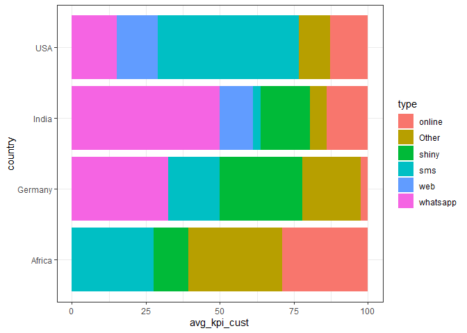
How to data wrangle and barplot the proportion without undesired stripes

Please find the input data and expected output as screenshot below:

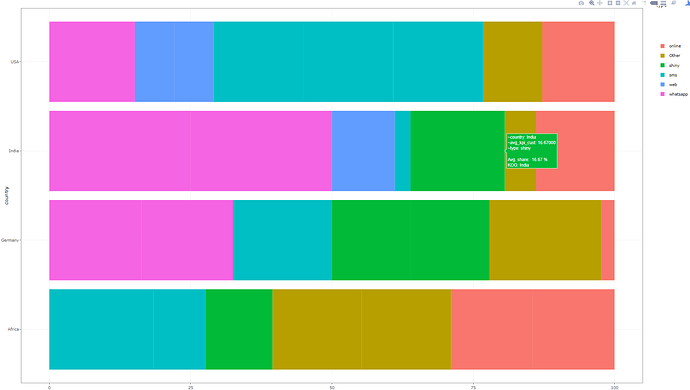
However, the current plot with the below code:

I feel, I made it too complicated. But I shared input data and expected data along with struggled code along the way. Could you please help us


# Input data
df <- tibble(
  country = c(rep(c("India","USA","Germany","Africa"), each = 8)),
  type = c("sms","Other","whatsapp","web","online","shiny","whatsapp","whatsapp",
              "sms","sms","sms","web","web","Other","online","whatsapp",
              "sms","Other","whatsapp","shiny","online","shiny","whatsapp","whatsapp",
              "sms","sms","sms","shiny","online","Other","online","Other"
  ),
  cust = rep(c("google","Apple","wallmart","pg"),8),
  quantity = c(10,20,30,40,50,60,70,80,
               90,100,15,25,35,45,55,65,
               75,85,95,105,10,15,20,25,
               30,35,40,45,50,55,60,65)
)

# Without Customer
df %>% 
  group_by(country,type) %>%
  summarise(kpi_wo_cust = sum(quantity)) %>% 
  ungroup() -> df_wo_cust

# With Customer
df %>% 
  group_by(country,type,cust) %>%
  summarise(kpi_cust = sum(quantity)) %>% 
  ungroup() -> df_cust

df_combo <- left_join(df_cust, df_wo_cust, by = c("country","type"))
df_combo %>% glimpse()

# Aggregated data for certain KPIs for final plot
df_aggr <- df_combo %>% 
  group_by(country,type) %>%
  mutate(kpi_cust_total = sum(kpi_cust),
         per_kpi_cust = 100 * (kpi_cust/kpi_cust_total)) %>%
  group_by(country) %>%
  # In order to except from repeated counting, selecting unique()
  mutate(kpi_cust_uniq_total = sum(kpi_cust) %>% unique(),
         per_unq_kpi_cust = 100 * (kpi_cust/kpi_cust_uniq_total) %>% round(4)) 

#
plt = df_aggr %>% ungroup() %>%#glimpse()

# In order to obtain theTop 2 customers (Major contributor) within country and type 
# However, if this code is used, there is an error
# group_by(country, type) %>%
 # nest()  %>%
 # mutate(top_cust = purrr::map_chr(data, function(x){
 #   x %>% arrange(desc(per_kpi_cust)) %>%
 #     top_n(2,per_kpi_cust) %>%
 #     summarise(Cust = paste(cust,round(per_kpi_cust,2), collapse = "<br>")) %>%
 #     pull(cust)
 # })#,data = NULL
 # ) %>%
 # unnest(cols = data) %>%
  group_by(country, type) %>%
# If mutate is used, undesired stripes appear on the plot 
  # Summarize used, then it is not adding to 100% 
  mutate(avg_kpi_cust = per_unq_kpi_cust %>% mean()) %>%
  #summarise(avg_kpi_cust = per_unq_kpi_cust %>% mean()) %>%
  ggplot(aes(x = country, 
             y = avg_kpi_cust, 
             fill = type,  
             text = paste('<br>proportion: ', round(avg_kpi_cust,2), "%",
                          "<br>country:",country
                          ))) +
  geom_bar(stat = "identity"#, position=position_dodge()
  ) +
  coord_flip() +
  theme_bw()


ggplotly(plt)
Hello!

It was kind of hard to understand what you were asking so I assumed you want the lines in each box gone. These are there because you group_by() cust. If you look at the data you are feeding into ggplot() there are multiple rows of each country, which results in those lines in ggplot. Removing cust in from the "with customer" will remove these lines. Reprex below!

Note: I added a comment noting where I removed cust

library(tidyverse)
#> Warning: package 'purrr' was built under R version 3.6.2
library(plotly)
#> 
#> Attaching package: 'plotly'
#> The following object is masked from 'package:ggplot2':
#> 
#>     last_plot
#> The following object is masked from 'package:stats':
#> 
#>     filter
#> The following object is masked from 'package:graphics':
#> 
#>     layout

# Input data
df <- tibble(
  country = c(rep(c("India","USA","Germany","Africa"), each = 8)),
  type = c("sms","Other","whatsapp","web","online","shiny","whatsapp","whatsapp",
           "sms","sms","sms","web","web","Other","online","whatsapp",
           "sms","Other","whatsapp","shiny","online","shiny","whatsapp","whatsapp",
           "sms","sms","sms","shiny","online","Other","online","Other"
  ),
  cust = rep(c("google","Apple","wallmart","pg"),8),
  quantity = c(10,20,30,40,50,60,70,80,
               90,100,15,25,35,45,55,65,
               75,85,95,105,10,15,20,25,
               30,35,40,45,50,55,60,65)
)

# Without Customer
df %>% 
  group_by(country,type) %>%
  summarise(kpi_wo_cust = sum(quantity)) %>% 
  ungroup() -> df_wo_cust

# With Customer
df %>% 
  group_by(country,type) %>% ## Remove cust
  summarise(kpi_cust = sum(quantity)) %>% 
  ungroup() -> df_cust

df_combo <- left_join(df_cust, df_wo_cust, by = c("country","type"))
df_combo %>% glimpse()
#> Observations: 20
#> Variables: 4
#> $ country     <chr> "Africa", "Africa", "Africa", "Africa", "Germany",...
#> $ type        <chr> "online", "Other", "shiny", "sms", "online", "Othe...
#> $ kpi_cust    <dbl> 110, 120, 45, 105, 10, 85, 120, 75, 140, 50, 20, 6...
#> $ kpi_wo_cust <dbl> 110, 120, 45, 105, 10, 85, 120, 75, 140, 50, 20, 6...

# Aggregated data for certain KPIs for final plot
df_aggr <- df_combo %>% 
  group_by(country,type) %>%
  mutate(kpi_cust_total = sum(kpi_cust),
         per_kpi_cust = 100 * (kpi_cust/kpi_cust_total)) %>%
  group_by(country) %>%
  # In order to except from repeated counting, selecting unique()
  mutate(kpi_cust_uniq_total = sum(kpi_cust) %>% unique(),
         per_unq_kpi_cust = 100 * (kpi_cust/kpi_cust_uniq_total) %>% round(4)) 

#
plt = df_aggr %>% ungroup() %>%#glimpse()
  
  # In order to obtain theTop 2 customers (Major contributor) within country and type 
  # However, if this code is used, there is an error
  # group_by(country, type) %>%
  # nest()  %>%
  # mutate(top_cust = purrr::map_chr(data, function(x){
  #   x %>% arrange(desc(per_kpi_cust)) %>%
  #     top_n(2,per_kpi_cust) %>%
  #     summarise(Cust = paste(cust,round(per_kpi_cust,2), collapse = "<br>")) %>%
  #     pull(cust)
  # })#,data = NULL
# ) %>%
# unnest(cols = data) %>%
group_by(country, type) %>%
  # If mutate is used, undesired stripes appear on the plot 
  # Summarize used, then it is not adding to 100% 
  mutate(avg_kpi_cust = per_unq_kpi_cust %>% mean()) %>%
  #summarise(avg_kpi_cust = per_unq_kpi_cust %>% mean()) %>%
  ggplot(aes(x = country, 
             y = avg_kpi_cust, 
             fill = type,  
             text = paste('Proportion: ', round(avg_kpi_cust,2), "%",
                          "<br>Country:", country
             ))) +
  geom_bar(stat = "identity"#, position=position_dodge()
  ) +
  coord_flip() +
  theme_bw()

plt

Created on 2020-02-03 by the reprex package (v0.3.0)

For the plotly call I would do ggplotly(plt, tooltip = "text"), this will remove the old tooltip and show the clean tooltip you were trying to make :slight_smile:

Thanks for your reply.
The idea behind adding cust in the grouping variable above is to obtain the proportion/contribution of cust within type.
If we remove "cust" then there will be no reason to create df_combo because df_cust and df_wo_cust are same. Also, ggplotly text has no value without cust grouping.

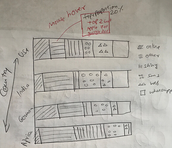
As sketched in the screenshot, top 2 cust are to be seen within ggplotly.

The key was to use distinct() after mutate() instead of summarise()
Also, mean() was the wrong function used earlier instead of sum() which had resulted in incomplete barplot.

library(tidyverse)
library(plotly)

# Input data
df <- tibble(
  country = c(rep(c("India","USA","Germany","Africa"), each = 8)),
  type = c("sms","Other","whatsapp","web","online","shiny","whatsapp","whatsapp",
              "sms","sms","sms","web","web","Other","online","whatsapp",
              "sms","Other","whatsapp","shiny","online","shiny","whatsapp","whatsapp",
              "sms","sms","sms","shiny","online","Other","online","Other"
  ),
  cust = rep(c("google","Apple","wallmart","pg"),8),
  quantity = c(10,20,30,40,50,60,70,80,
               90,100,15,25,35,45,55,65,
               75,85,95,105,10,15,20,25,
               30,35,40,45,50,55,60,65)
)

# Without Customer
df %>% 
  group_by(country,type) %>%
  summarise(kpi_wo_cust = sum(quantity)) %>% 
  ungroup() -> df_wo_cust

# With Customer
df %>% 
  group_by(country,type,cust) %>%
  summarise(kpi_cust = sum(quantity)) %>% 
  ungroup() -> df_cust

df_combo <- left_join(df_cust, df_wo_cust, by = c("country","type"))
df_combo %>% glimpse()

# Aggregated data for certain KPIs for final plot
df_aggr <- df_combo %>% 
  group_by(country,type) %>%
  mutate(kpi_cust_total = sum(kpi_cust),
         per_kpi_cust = 100 * (kpi_cust/kpi_cust_total)) %>%
  group_by(country) %>%
  # In order to except from repeated counting, selecting unique()
  mutate(kpi_cust_uniq_total = sum(kpi_cust) %>% unique(),
         per_unq_kpi_cust = 100 * (kpi_cust/kpi_cust_uniq_total) %>% round(4)) 

plt = df_aggr %>% ungroup() %>%
# In order to diplay Top 2 customers (Major contributor) within country and type 
group_by(country, type) %>%
nest()  %>%
mutate(top_cust = purrr::map_chr(data, function(x){
  x %>% arrange(desc(per_kpi_cust)) %>%
    top_n(2,per_kpi_cust) %>%
    summarise(Cust = paste(cust,round(per_kpi_cust,2), collapse = "<br>")) %>%
    pull(Cust)
})) %>%
unnest(cols = data) %>%
  group_by(country, type) %>%
# If mutate is used, undesired stripes appear on the plot 
  # Summarize used, then it is not adding to 100%.
  # So distinct was used
  mutate(avg_kpi_cust = per_unq_kpi_cust %>% sum()) %>%
  ungroup() %>%
  distinct(country, type, .keep_all = T) %>%
  ggplot(aes(x = country, 
             y = avg_kpi_cust, 
             fill = type,  
             text = top_cust
                          )) +
  geom_bar(stat = "identity") +
  coord_flip() +
  theme_bw()

ggplotly(plt, tooltip = "text")

This topic was automatically closed 7 days after the last reply. New replies are no longer allowed.