How to crop gridded data with shapefile

[Ellenz]

Dear ggplot2 users,
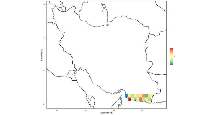
I plot the gridded data with ggplot2 as in the figure (as an example). The gridded dataset is like DFgrid. The outside black boundary in the figure is a shapefile of the study area. How to crop the gridded data with the shapefile, so that the gridded data can perfectly be bounded inside of the black boundary? I could not find any source for this. Thanks for your help.

By the way, the figure does not represent the data, but I made an
My problem is, how to crop the gridded data, so that the gridded data only shows inside the boundary but not outside of the boundary. The gridded data follows the curve of the shapefile boundary. Thanks.

[andresrcs]

As usual, could you please turn this into a proper REPRoducible EXample (reprex)?

[Ellenz]

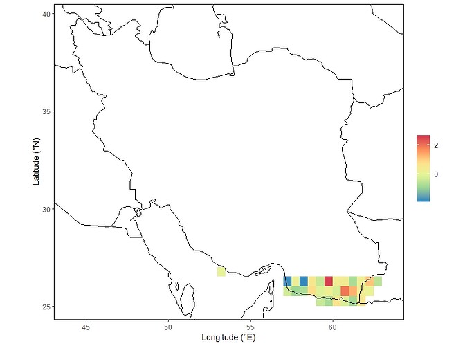
I don't know how to upload the shapefile, so the data, code and figure are shown below. Due to the large volume of the DFgrid file, I only included part of the dataset, but the dataframe structure is the same. The DFgrid covers whole shapefile border, but some grids are even outside of the border. I can only draw the two figures separately. How to crop the DFgrid file to the shapefile border, so that all grids are inside of the border and have perfect curves at the verge? I would really appreciate your help.

######################### example file

library(ggplot2)

DFgrid= data.frame(
  lon=c(59.25, 59.75, 60.25, 60.75, 61.25, 61.75, 57.25, 57.75, 58.25, 58.75, 59.25, 59.75, 60.25, 60.75, 61.25, 61.75, 62.25, 57.25, 57.75, 58.25, 58.75, 59.25, 59.75, 60.25, 60.75, 61.25, 61.75, 62.25, 62.75, 53.25),
  lat=c(25.25, 25.25, 25.25, 25.25, 25.25, 25.25, 25.75, 25.75, 25.75, 25.75, 25.75, 25.75, 25.75, 25.75, 25.75, 25.75, 25.75, 26.25, 26.25, 26.25, 26.25, 26.25, 26.25, 26.25, 26.25, 26.25, 26.25, 26.25, 26.25, 26.75),
  value= rnorm(30)
)

my_year <- theme_bw() + theme(panel.ontop=TRUE, panel.background=element_blank())
my_fill <- scale_fill_distiller('',palette='Spectral',
                                breaks = c(-2,0,2))

fig = ggplot(DFgrid, aes(y=lat, x=lon, fill=value)) + geom_tile() + my_year + my_fill+
  coord_quickmap(xlim=c(44.05, 63.35), ylim=c(25.05, 39.75))+
  borders('world', xlim=c(44.05, 63.35), ylim=c(25.05, 39.75), colour='black')+
  xlab('Longitude (°E)')+ ylab('Latitude (°N)')+
  theme(panel.grid=element_blank(),
        panel.border = element_rect(colour = "black", fill=NA,size=.7))
print(fig)

 install.packages("maptools",repos="http://cran.us.r-project.org")
> library(maptools)
> library(rgdal)
> library(raster)
> setwd('C:/Users/Acer/Desktop/border_shape')
> list.files()
[1] "border.CPG"     "border.dbf"     "border.prj"     "border.shp"     "border.shp.xml"
[6] "border.shx"    
> data.shape<-readOGR(dsn=".",layer="border")
OGR data source with driver: ESRI Shapefile 
Source: "C:\Users\Acer\Desktop\border_shape", layer: "border"
with 1 features
It has 70 fields
Integer64 fields read as strings:  ID_0 OBJECTID_1 
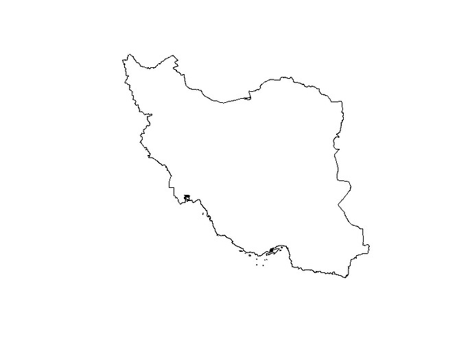
> plot(data.shape)
> class(data.shape)  # Describes the type of vector data stored in the object.
[1] "SpatialPolygonsDataFrame"
attr(,"package")
[1] "sp"
> length(data.shape)  # How many features are in this spatial object?
[1] 1
> extent(data.shape)  # The spatial extent (geographic area covered by) features in the object.
class       : Extent 
xmin        : 44.04726 
xmax        : 63.31746 
ymin        : 25.05875 
ymax        : 39.77722 
> crs(data.shape)  # coordinate reference system
CRS arguments:
 +proj=longlat +datum=WGS84 +no_defs +ellps=WGS84 +towgs84=0,0,0 
 Plot it
> data.shape = readOGR(dsn='C:/Users/Acer/Desktop/border_shape/.',layer='border')
OGR data source with driver: ESRI Shapefile 
Source: "C:\Users\Acer\Desktop\border_shape", layer: "border"
with 1 features
It has 70 fields
Integer64 fields read as strings:  ID_0 OBJECTID_1 
> plot(data.shape)

[jlacko]

I believe you are looking for a combination of raster::mask() and possibly raster::crop().

Have a look at this answer from a while back, it seems the issue is similar.

temperature maps in R

I can not reproduce your code, but allow me to illustrate the approach on a similar use case; I have used temperature data from Copernicus and cropped it to shape of the Czech Republic from GADM. This approach requires only two packages (raster and sf) + tidyverse, just because :)) It uses two steps: remove the extra data points via raster::mask() crop the file down to size via raster::crop() library(tidyverse) # because tidyverse library(raster) # raster spatial data processing library(sf) # vector spatial data processing data <- raster("./src/tg_0.25deg_day_2019_grid_ensmean.nc") # your ncdf file borders <- readRDS("./src/gadm36_CZE_0_sf.rds") # country borders in sf …

Also note that you will be better off with reading the country polygon in with sf::st_read(), as the {sf} package format is newer and IMHO more user friendly than the older {sp}.

[Ellenz]

Thanks for your reply. But my problem is a little different. (1) I do not have the nc file, but rather I have the txt file to plot. I used ggplot then, and didn't convert the txt file to raster. (2) How to convert the .shp file to a sf format?
So how to do this? Thanks.

[jlacko]

The data you have are raster data (evenly spaced grid, with values). The nc is just one of many variations of that.

I believe you should be able to convert the data frame to {raster} format by calling

raster_frame <- raster::rasterFromXYZ(DFgrid)

and perform your croping & masking.

Then you will need something like this to get the cropped raster to ggplot friendly format again.

raster_frame <- raster_frame %>%  
  as("SpatialPixelsDataFrame") %>% 
  as_data_frame()

fig <- ggplot() + geom_tile(data = raster_frame, aes(x = x, y = y, fill = value)) + my_year + my_fill+
  coord_quickmap(xlim=c(44.05, 63.35), ylim=c(25.05, 39.75))+
  borders('world', xlim=c(44.05, 63.35), ylim=c(25.05, 39.75), colour='black')+
  xlab('Longitude (°E)')+ ylab('Latitude (°N)')+
  theme(panel.grid=element_blank(),
        panel.border = element_rect(colour = "black", fill=NA,size=.7))
print(fig)

[Ellenz]

How to do the crop and mask? I tried the code below, but got the warning message

#### get the cropped raster to ggplot friendly format again.
> raster_frame <- raster_frame %>%  
>   as("SpatialPixelsDataFrame") %>% 
>   as_data_frame()

> Error in as(., "SpatialPixelsDataFrame") : 
>   no method or default for coercing “tbl_df” to “SpatialPixelsDataFrame”

[jlacko]

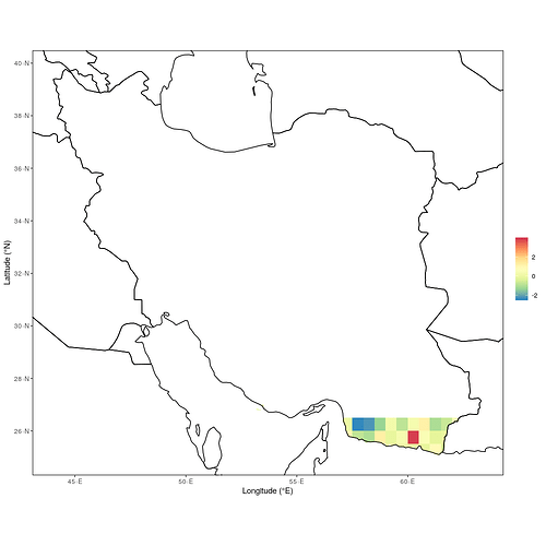
As your shapefile seems to be of a country politely referred to as Persia I suggest the following code.

It downloads the shape of Iran from GADM and crops your data to the shape via raster::mask()

I had to tweak your ggplot code a bit (replacing lat / lon with x / y) but otherwise it is the same code.

library(tidyverse)
library(raster)
library(sf)

borders <- readRDS(url("https://biogeo.ucdavis.edu/data/gadm3.6/Rsf/gadm36_IRN_0_sf.rds"))

DFgrid <- data.frame(
  lon=c(59.25, 59.75, 60.25, 60.75, 61.25, 61.75, 57.25, 57.75, 58.25, 58.75, 59.25, 59.75, 60.25, 60.75, 61.25, 61.75, 62.25, 57.25, 57.75, 58.25, 58.75, 59.25, 59.75, 60.25, 60.75, 61.25, 61.75, 62.25, 62.75, 53.25),
  lat=c(25.25, 25.25, 25.25, 25.25, 25.25, 25.25, 25.75, 25.75, 25.75, 25.75, 25.75, 25.75, 25.75, 25.75, 25.75, 25.75, 25.75, 26.25, 26.25, 26.25, 26.25, 26.25, 26.25, 26.25, 26.25, 26.25, 26.25, 26.25, 26.25, 26.75),
  value= rnorm(30)
)

raster_frame <- rasterFromXYZ(DFgrid) %>% 
  mask(borders) %>% 
  as("SpatialPixelsDataFrame") %>% 
  as_data_frame()

my_year <- theme_bw() + theme(panel.ontop=TRUE, panel.background=element_blank())
my_fill <- scale_fill_distiller('',palette='Spectral',
                                breaks = c(-2,0,2))

fig = ggplot() + geom_tile(data = raster_frame, aes(x=x, y=y, fill=value)) + my_year + my_fill+
  coord_quickmap(xlim=c(44.05, 63.35), ylim=c(25.05, 39.75))+
  borders('world', xlim=c(44.05, 63.35), ylim=c(25.05, 39.75), colour='black')+
  xlab('Longitude (°E)')+ ylab('Latitude (°N)')+
  theme(panel.grid=element_blank(),
        panel.border = element_rect(colour = "black", fill=NA,size=.7))
print(fig)

[Ellenz]

Thanks. It looks better, but some grids still straddle the border. Is it possible to cut the grids at the border to the shape fits the border?

[jlacko]

It really depends on what you want to achieve.

• You can either do the selection at the data level, and discard the grid cells that are not entirely contained by the country borders. This is good if you want to do some calculation on the resulting raster, but the cells look somewhat ragged.
• Or you can keep the data as they are, and keep all the action at the plotting level = overlay the grid cells with a white mask cut to the shape of country borders. The data will remain as they were, but the plot will be nice & even.

The first option - built on raster::mask() - is in my code sample above.

The second, masking, does not require {raster} and makes do with {sf} only:

library(tidyverse)
library(sf)

borders <- readRDS(url("https://biogeo.ucdavis.edu/data/gadm3.6/Rsf/gadm36_IRN_0_sf.rds"))

DFgrid <- data.frame(
   lon=c(59.25, 59.75, 60.25, 60.75, 61.25, 61.75, 57.25, 57.75, 58.25, 58.75, 59.25, 59.75, 60.25, 60.75, 61.25, 61.75, 62.25, 57.25, 57.75, 58.25, 58.75, 59.25, 59.75, 60.25, 60.75, 61.25, 61.75, 62.25, 62.75, 53.25),
   lat=c(25.25, 25.25, 25.25, 25.25, 25.25, 25.25, 25.75, 25.75, 25.75, 25.75, 25.75, 25.75, 25.75, 25.75, 25.75, 25.75, 25.75, 26.25, 26.25, 26.25, 26.25, 26.25, 26.25, 26.25, 26.25, 26.25, 26.25, 26.25, 26.25, 26.75),
   value= rnorm(30)
)


mask <- borders %>% 
   st_bbox() %>% 
   st_as_sfc() %>% 
   st_buffer(5) %>% 
   st_difference(borders) %>% 
   st_as_sf()


my_year <- theme_bw() + theme(panel.ontop=TRUE, panel.background=element_blank())
my_fill <- scale_fill_distiller('',palette='Spectral',
                                breaks = c(-2,0,2))

fig = ggplot() + geom_tile(data = DFgrid, aes(y=lat, x=lon, fill=value)) + my_year + my_fill +
   geom_sf(data = mask, fill = "white", color = NA) +
   coord_sf(xlim=c(44.05, 63.35), ylim=c(25.05, 39.75)) +
   borders('world', xlim=c(44.05, 63.35), ylim=c(25.05, 39.75), colour='black')+
   xlab('Longitude (°E)')+ ylab('Latitude (°N)')+
   theme(panel.grid=element_blank(),
         panel.border = element_rect(colour = "black", fill=NA,size=.7))

print(fig)

The final choice is up to you

[Ellenz]

Thanks, I want to achieve the second option. But I got the error message when making the 'mask' file. How to solve this? Thanks.

mask <- borders %>%
st_bbox() %>%
st_as_sfc() %>%
st_buffer(5) %>%
st_difference(borders) %>%
st_as_sf()

dist is assumed to be in decimal degrees (arc_degrees).
although coordinates are longitude/latitude, st_difference assumes that they are planar
Error in UseMethod("st_as_sf") :
no applicable method for 'st_as_sf' applied to an object of class "c('sfc_POLYGON', 'sfc')"
In addition: Warning message:
In st_buffer.sfc(., 5) :
st_buffer does not correctly buffer longitude/latitude data

[jlacko]

The messages are more like warnings than errors. They basically tell you that your map is flat, while the world is not.

At this level of detail they can be safely ignored; they should have no effect on the plot (there might be a minor inconsistency on edges if the GADM shapefile is simplified differently than the one used by ggplot2::borders ())

[Ellenz]

There is problem, actually. When I ran the script to make the ggplot, it could not go through:

Error in geom_sf(data = mask, fill = "white", color = NA) :
object 'mask' not found

[jlacko]

That is strange... It implies there is something with your {sf} package (or dependencies). Try updating it.
Are you on Linux by chance?

[Ellenz]

No, I'm not on Linux. I tried both on mac and windows, and got the same error. I will update first. This updating method seems not the right way.

update.packages('sf')

Thanks.

[jlacko]

If update.packages("sf") does not help you might reinstall it - remove.packages("sf") and then install.packages("sf").

[Ellenz]

Yes, there is a problem with the package itself. For example, I tried to remove it and then install it, but it says:

Warning in install.packages :
installation of package ‘sf’ had non-zero exit status

[jlacko]

So I suspected

What error message did you get? Something about required library missing?

[Ellenz]

Here is the process below. I am not very aware of the problems...

> install.packages("sf")
also installing the dependency ‘classInt’


  There are binary versions available but the source versions
  are later:
         binary source needs_compilation
classInt  0.3-1  0.4-1              TRUE
sf        0.7-3  0.8-0              TRUE

Do you want to install from sources the packages which need compilation?
y/n: y
installing the source packages ‘classInt’, ‘sf’

trying URL 'https://cloud.r-project.org/src/contrib/classInt_0.4-1.tar.gz'
Content type 'application/x-gzip' length 19048 bytes (18 KB)
==================================================
downloaded 18 KB

trying URL 'https://cloud.r-project.org/src/contrib/sf_0.8-0.tar.gz'
Content type 'application/x-gzip' length 8607770 bytes (8.2 MB)
==================================================
downloaded 8.2 MB

* installing *source* package ‘classInt’ ...
** package ‘classInt’ successfully unpacked and MD5 sums checked
** libs
gfortran   -fPIC  -g -O2  -c fish1.f -o fish1.o
make: gfortran: No such file or directory
make: *** [fish1.o] Error 1
ERROR: compilation failed for package ‘classInt’
* removing ‘/Library/Frameworks/R.framework/Versions/3.4/Resources/library/classInt’
* restoring previous ‘/Library/Frameworks/R.framework/Versions/3.4/Resources/library/classInt’
Warning in install.packages :
  installation of package ‘classInt’ had non-zero exit status
* installing *source* package ‘sf’ ...
** package ‘sf’ successfully unpacked and MD5 sums checked
configure: CC: clang
configure: CXX: clang++ -std=gnu++11
checking for gdal-config... no
no
configure: error: gdal-config not found or not executable.
ERROR: configuration failed for package ‘sf’
* removing ‘/Library/Frameworks/R.framework/Versions/3.4/Resources/library/sf’
Warning in install.packages :
  installation of package ‘sf’ had non-zero exit status

The downloaded source packages are in
	‘/private/var/folders/rs/dzg78fb95339szp7hlnrrc6m0000gn/T/RtmpPnp2fc/downloaded_packages’
> library(sf)
Error in library(sf) : there is no package called ‘sf’

[jlacko]

Try installing the binaries; you don't need the very latest features and compiling from source can be tricky.
(that is why I asked about Linux; you have to compile from source on Linux)