I know how to create an interaction plot of the factors I have in my data frame, but once I have set up contrasts, how do I plot interaction plot according to the contrasts I set?
Is there a function I can use?
Thanks.
I know how to create an interaction plot of the factors I have in my data frame, but once I have set up contrasts, how do I plot interaction plot according to the contrasts I set?
Is there a function I can use?
Thanks.
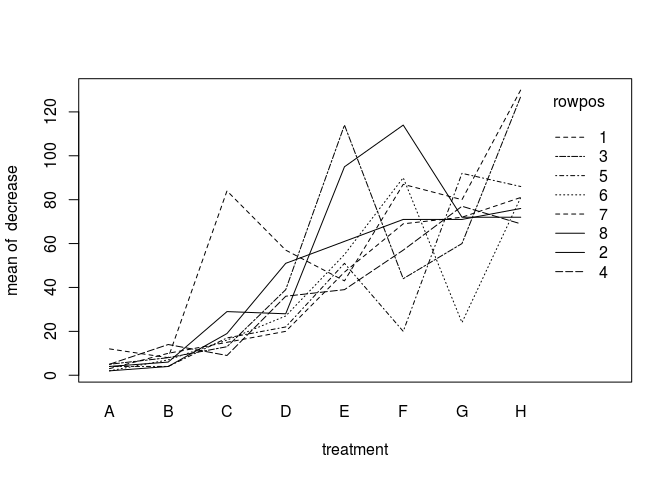
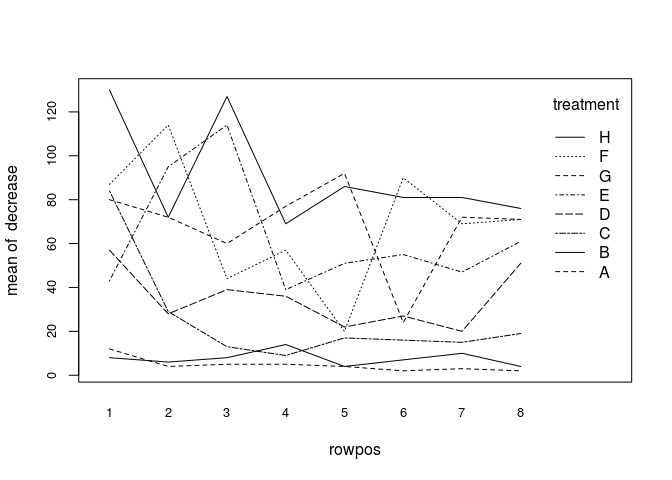
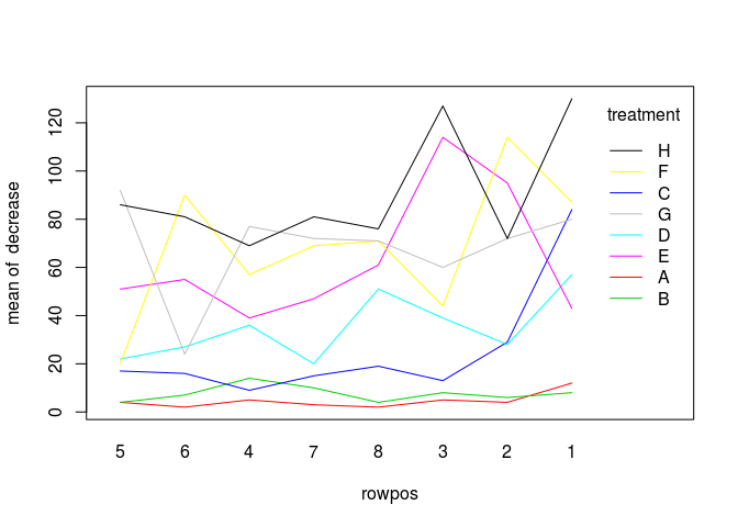
Can you give us an example of what you mean by "set up contrasts"? Below is an example from the interaction.plot help file. Maybe start with that and make an reproducible example so we can better help you out.
require(graphics)


with(OrchardSprays, {
interaction.plot(treatment, rowpos, decrease)
interaction.plot(rowpos, treatment, decrease, cex.axis = 0.8)
## order the rows by their mean effect
rowpos <- factor(rowpos,
levels = sort.list(tapply(decrease, rowpos, mean)))
interaction.plot(rowpos, treatment, decrease, col = 2:9, lty = 1)
})


For example, I have factor A with a1 and a2, two levels, and factor B with b1 and b2 and b3, three levels.
I know how to create an interaction plot.
But once I set my own contrast
A <-- c(-1, 1)
contrasts(B) <-- cbine(c(-2, 1, 1), c(0, -1, 1))
How do I plot the interaction plot of A and B according to the two contrasts I set for B?
You're going to find it really hard to get help without a reproducible example that contains executable R code:
Thank you very much. I will provide a reproducible example.
http://localhost:21290/session/fileffc74fafb411_reprex.html
I don't know how to paste it here. Can you see the codes, or can you teach me how to post the codes I created here?
Sorry for the fundamental questions, I am trying to learn R.
Can you give us the code you used which is describing the behavior you are trying to solve? If you have issues figuring out how to share your dataframe, you install the package datapasta which can allow you to re-create runable code via the following:
install.packages("datapasta")
#Below will output the object, and assign it to df
df <- datapasta::tribble_paste(mtcars)
Let us know if you have further issues.
What I am asking is I know how to create an interaction plot between my two factors: gender and alcohol, however, if I want to create two interaction plots, each represents the contrasts I set (i.e. No alcohol v.s Average of Alcohol between gender, and 2 Pints v.s. 4 Pints between gender), is there a function or anyway I can use to do so?
(I figure out I can just paste it here. My code and the plot in my textbook I am trying to create are in the next post. Sorry for being so dumb and slow to figure out such simple thing.)
library(car)
#> Warning: package 'car' was built under R version 3.4.4
#> Loading required package: carData
library(compute.es)
library(effects)
#> lattice theme set by effectsTheme()
#> See ?effectsTheme for details.
library(ggplot2)
library(multcomp)
#> Loading required package: mvtnorm
#> Loading required package: survival
#> Loading required package: TH.data
#> Loading required package: MASS
#>
#> Attaching package: 'TH.data'
#> The following object is masked from 'package:MASS':
#>
#>     geyser
library(pastecs)
#> Warning: package 'pastecs' was built under R version 3.4.4
library(reshape)
library(WRS2)
library(Hmisc)
#> Loading required package: lattice
#> Loading required package: Formula
#>
#> Attaching package: 'Hmisc'
#> The following objects are masked from 'package:base':
#>
#>     format.pval, units
library(Rcmdr)
#> Loading required package: splines
#> Loading required package: RcmdrMisc
#> Loading required package: sandwich
#>
#> Attaching package: 'RcmdrMisc'
#> The following object is masked from 'package:Hmisc':
#>
#>     Dotplot
#> The Commander GUI is launched only in interactive sessions
#>
#> Attaching package: 'Rcmdr'
#> The following object is masked from 'package:car':
#>
#>     Confint

#dataframe
gender <- gl(2, 24, labels = c("Female", "Male"))
alcohol <- gl(3, 8, 48, labels = c("None", "2 Pints", "4 Pints"))
attractiveness <- c(65,70,60,60,60,55,60,55,70,65,60,70,65,60,60,50,55,65,70,55,55,60,50,50,50,55,80,65,70,75,75,65,45,60,85,65,70,70,80,60,30,30,30,55,35,20,45,40)
gogglesData <- data.frame(gender, alcohol, attractiveness)
gogglesData
#>    gender alcohol attractiveness
#> 1  Female    None             65
#> 2  Female    None             70
#> 3  Female    None             60
#> 4  Female    None             60
#> 5  Female    None             60
#> 6  Female    None             55
#> 7  Female    None             60
#> 8  Female    None             55
#> 9  Female 2 Pints             70
#> 10 Female 2 Pints             65
#> 11 Female 2 Pints             60
#> 12 Female 2 Pints             70
#> 13 Female 2 Pints             65
#> 14 Female 2 Pints             60
#> 15 Female 2 Pints             60
#> 16 Female 2 Pints             50
#> 17 Female 4 Pints             55
#> 18 Female 4 Pints             65
#> 19 Female 4 Pints             70
#> 20 Female 4 Pints             55
#> 21 Female 4 Pints             55
#> 22 Female 4 Pints             60
#> 23 Female 4 Pints             50
#> 24 Female 4 Pints             50
#> 25   Male    None             50
#> 26   Male    None             55
#> 27   Male    None             80
#> 28   Male    None             65
#> 29   Male    None             70
#> 30   Male    None             75
#> 31   Male    None             75
#> 32   Male    None             65
#> 33   Male 2 Pints             45
#> 34   Male 2 Pints             60
#> 35   Male 2 Pints             85
#> 36   Male 2 Pints             65
#> 37   Male 2 Pints             70
#> 38   Male 2 Pints             70
#> 39   Male 2 Pints             80
#> 40   Male 2 Pints             60
#> 41   Male 4 Pints             30
#> 42   Male 4 Pints             30
#> 43   Male 4 Pints             30
#> 44   Male 4 Pints             55
#> 45   Male 4 Pints             35
#> 46   Male 4 Pints             20
#> 47   Male 4 Pints             45
#> 48   Male 4 Pints             40

#interaction plot
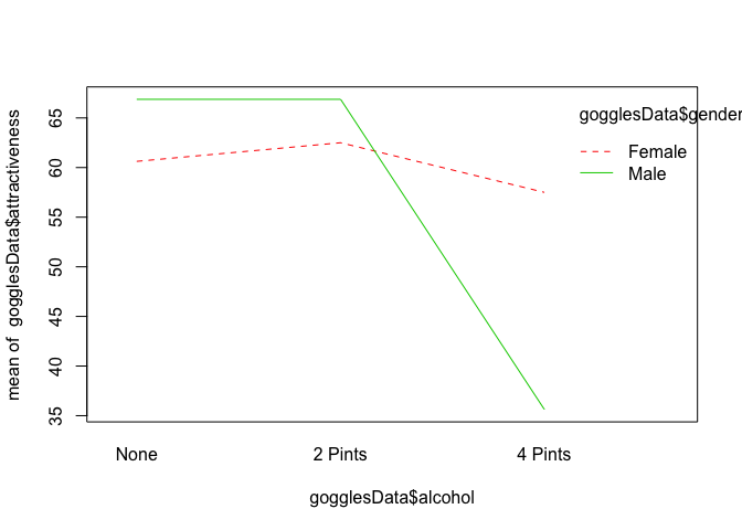
interaction.plot(gogglesData$alcohol, gogglesData$gender, gogglesData$attractiveness, col = 2:3)

#ANOVA
contrasts(gogglesData$alcohol) <- cbind(c(-2, 1, 1), c(0, -1, 1))
contrasts(gogglesData$gender) <- c(-1, 1)
gogglesModel <- aov(attractiveness ~ gender*alcohol, data = gogglesData)
Anova(gogglesModel, type="III")
#> Anova Table (Type III tests)
#>
#> Response: attractiveness
#>                Sum Sq Df   F value    Pr(>F)
#> (Intercept)    163333  1 1967.0251 < 2.2e-16 ***
#> gender            169  1    2.0323    0.1614
#> alcohol          3332  2   20.0654 7.649e-07 ***
#> gender:alcohol   1978  2   11.9113 7.987e-05 ***
#> Residuals        3488 42
#> ---
#> Signif. codes:  0 '***' 0.001 '**' 0.01 '*' 0.05 '.' 0.1 ' ' 1
Created on 2018-06-30 by the reprex package (v0.2.0).
And I am wondering how do I create these two plot in my textbook:
Thanks for your code.
Can you elaborate on what book you found this plot from? It looks like it may be created with ggplot2, but I think looking at where the chart was referenced could be a good starting point to figure out how to rebuild the chart you referenced.
It is from Andy Field's book, Discovering Statistics Using R, p.525, Figure 12.9.
And yes, it is created by ggplot2. I know how to use ggplot2 to create an interaction plot of the two factors, too, but I don't know if there's a function to create plots representing the contrasts as those in Figure 12.9.
I can actually use the following code to get these points I need, and to create these plots. But I am wondering if there's a faster or smarter way to do so.
Thanks for help. ![]()
#Interaction Plot
line <- ggplot(gogglesData, aes(alcohol, attractiveness, colour = gender))
line + stat_summary(fun.y = mean, geom = "point") + stat_summary(fun.y = mean, geom = "line", aes(group = gender)) + stat_summary(fun.data = mean_cl_boot, geom = "errorbar", width = 0.2) + labs(x = "Alcohol Consumption", y = "Mean Attractiveness of Date (%)")

interactionMeans <- allEffects(gogglesModel)
summary(interactionMeans)
#>  model: attractiveness ~ gender * alcohol
#>
#>  gender*alcohol effect
#>         alcohol
#> gender     None 2 Pints 4 Pints
#>   Female 60.625  62.500  57.500
#>   Male   66.875  66.875  35.625
#>
#>  Lower 95 Percent Confidence Limits
#>         alcohol
#> gender       None  2 Pints  4 Pints
#>   Female 54.12331 55.99831 50.99831
#>   Male   60.37331 60.37331 29.12331
#>
#>  Upper 95 Percent Confidence Limits
#>         alcohol
#> gender       None  2 Pints  4 Pints
#>   Female 67.12669 69.00169 64.00169
#>   Male   73.37669 73.37669 42.12669


Created on 2018-07-01 by the [reprex package](http://reprex.tidyverse.org) (v0.2.0).