How to compare a forecast model to actual data and what is uncertainty?

Hello all,

in my class we were told to run a forecast model based on ETS and ARIMA and then compare these models to the actual data. I have run the models, but I don't know how to compare them to the actual data. We also have to talk about the uncertainty represented in these models.
Can some one help me with how to run the comparison and explain what is the uncertainty?

thanks.

here is a reprex() of what I have so far, both of these models ran fine so I don't know why the reprex() is showing errors.


# arima instead of exp smooth
arimafit <- auto.arima(terror_byMonth)
#> Error in auto.arima(terror_byMonth): could not find function "auto.arima"

# fit exp smooth model
m_ets = ets(terror_byMonth) 
#> Error in ets(terror_byMonth): could not find function "ets"

# forecast ETS 2017
f_ets = forecast(m_ets, h=12) 
#> Error in forecast(m_ets, h = 12): could not find function "forecast"

# forecast ARIMA 2017
f_arima<-forecast(arimafit,h=12)
#> Error in forecast(arimafit, h = 12): could not find function "forecast"

# check accuracy ETS
ets_acc <- accuracy(m_ets) 
#> Error in accuracy(m_ets): could not find function "accuracy"

# check accuarcy ARIMA
arima_acc <- accuracy(arimafit)
#> Error in accuracy(arimafit): could not find function "accuracy"

# Compair to acctually 2017 data???
#????
#????

Created on 2019-02-11 by the reprex package (v0.2.1)
Homework inspired questions should come in the form of a reproducible example, your code is not reproducible because you are not including library calls and sample data, please read this FAQ about how to make a reprex.

Also, please make sure to follow our homework policy

Rather than try and work off your example, I'll try and give you a few tools in the forecast package for doing multi-step ahead forecasts, and for one-step ahead out of sample forecasts. This should give you some sense of the uncertainty in your model, and help you visualize performance.

Also, note how in my reproducible example, I load the packages and the data up top (the data comes from base R itself) so my script runs completely without any errors. You are missing the loading packages step, and we don't have access to your data either so we can't run your code.

library(ggplot2)
library(forecast)

data("AirPassengers")

# Through the end of 1956, but no months in 1957
air_train <- window(AirPassengers, end = 1956+11/12)

# everything in 1957 and on
air_test  <- window(AirPassengers, start = 1957)

n_test <- length(air_test)

# //////////////////////////////////////////////////////////////////////////////

# Fit model to first few years of AirPassengers data
air_model <- auto.arima(air_train)

# So we get an Arima model back
air_model
#> Series: air_train 
#> ARIMA(1,1,0)(1,1,0)[12] 
#> 
#> Coefficients:
#>           ar1     sar1
#>       -0.2250  -0.2274
#> s.e.   0.1076   0.1081
#> 
#> sigma^2 estimated as 92.5:  log likelihood=-304.98
#> AIC=615.97   AICc=616.27   BIC=623.22

# You can look at the "performance", but this is the in sample performance
# i.e. it is computing performance using the data that it was fit with
accuracy(air_model)
#>                     ME     RMSE      MAE       MPE     MAPE      MASE
#> Training set 0.4424643 8.834477 6.351387 0.1376786 2.870884 0.2174955
#>                     ACF1
#> Training set 0.003854251

# Its an "Arima" object
class(air_model)
#> [1] "ARIMA" "Arima"

# //////////////////////////////////////////////////////////////////////////////

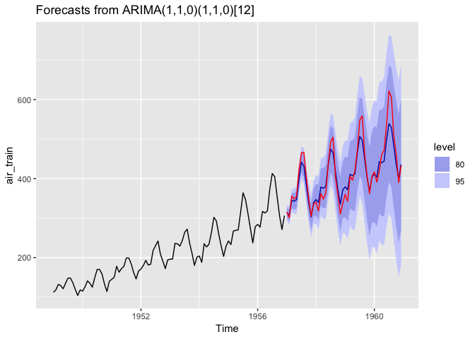
# We could do "multistep" forecasts for as many days are in the test set
# This repeatedly feeds the predicted data point back into the prediction
# equation to get the next prediction
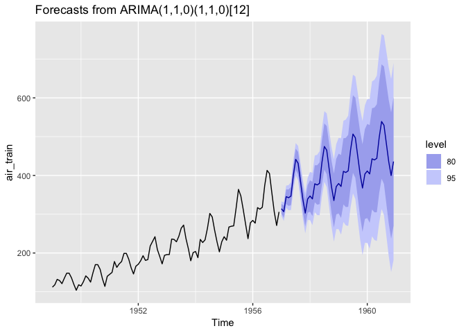
air_multi_forecast <- air_model %>%
  forecast(h = n_test)

air_multi_forecast %>%
  autoplot()


# You could compute performance using this and compare it to
# the test set. You can do that by passing a test set of the
# same size as the forecast to `x` in accuracy()
accuracy(air_multi_forecast, x = air_test)
#>                     ME      RMSE       MAE       MPE     MAPE      MASE
#> Training set 0.4424643  8.834477  6.351387 0.1376786 2.870884 0.2174955
#> Test set     6.8490404 26.471644 19.501243 0.8396151 4.405293 0.6677963
#>                     ACF1 Theil's U
#> Training set 0.003854251        NA
#> Test set     0.675272576 0.5053222

# And we can plot this
air_multi_forecast %>%
  autoplot() +
  geom_line(
    aes(
      x = as.numeric(time(air_test)),
      y = as.numeric(air_test)
    ),
    col = "red"
  )


# //////////////////////////////////////////////////////////////////////////////

# Apply ALREADY FIT model to NEW data
# This predicts "one step ahead" forecasts
# Basically:
# - Tomorrow's data point is predicted
# - The actual data point for tomorrow is added to the model prediction equation
# - The data point for 2 days from now is predicted using the updated info
# - And so on...
air_model_test <- Arima(air_test, model = air_model)

# Uses the same coef as the air_model. Nothing is actually "refit"
coef(air_model)
#>        ar1       sar1 
#> -0.2249847 -0.2273654
coef(air_model_test)
#>        ar1       sar1 
#> -0.2249847 -0.2273654

# When you call accuracy on this, you get "one step ahead"
# out of sample forecasts
accuracy(air_model_test)
#>                     ME     RMSE      MAE         MPE     MAPE      MASE
#> Training set 0.2893967 13.44907 8.868658 -0.01146318 2.057566 0.2469232
#>                    ACF1
#> Training set -0.1944196

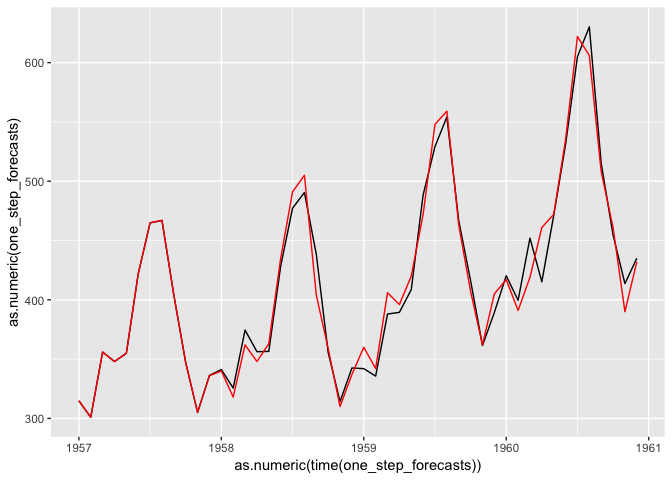
# Extract the actual 1 step forecast values
one_step_forecasts <- fitted(air_model_test)

# This is really ugly but whatever
# Compare this to the previous plot and you can see that
# the errors are not as extreme as before. This is because
# you are continually updating the prediction equation with
# new data. So you don't propogate uncertainty from a bad
# forecast about tomorrow into the forecast for the next
# day
ggplot() +
  geom_line(
    aes(
      x = as.numeric(time(one_step_forecasts)),
      y = as.numeric(one_step_forecasts)
    ),
    col = "black"
  ) +
  geom_line(
    aes(
      x = as.numeric(time(air_test)),
      y = as.numeric(air_test)
    ),
    col = "red"
  )


# //////////////////////////////////////////////////////////////////////////////

# There is a third way that I can describe but won't show.
# Rather than simply updating the prediction equation with the new data
# point, and NOT changing the model coefficients, you can actually do a 
# full refit of the model each time you get a new data point and then predict
# with that. This makes sense in some scenarios, and you can compare this 
# method to using the simple one step ahead approach I showed above as a
# way to see how stable your model coefficients are.
3 Likes

Thank you so much!

These are exactly the kinds of examples I've been looking for!

Okay here's a reprex() of my script. I included the last three years (36 rows) of the data I'm working with. Reprex still shows errors, but the file: "globalterrorismdb_0718dist.csv" is in my directory. Likewise, I had previously checked each of the libraries from the "packages" tap in rStudio. I put them explicitly in the script this time. I'm assuming these errors are because I'm not using data() for my data set. Is this correct?

# Author: Sal Meza
# Data Science 489/ Spring
# Data: 2/11/19
# last modified: 2/11/19

library(ggplot2)
library(forecast)
library(tseries)
library(reprex)

pastaTerror <- tibble::tribble(
              ~imonth, ~iyear, ~monthly,
                    1,   2015,     1534,
                    2,   2015,     1295,
                    3,   2015,     1183,
                    4,   2015,     1277,
                    5,   2015,     1316,
                    6,   2015,     1168,
                    7,   2015,     1263,
                    8,   2015,     1290,
                    9,   2015,     1107,
                   10,   2015,     1269,
                   11,   2015,     1172,
                   12,   2015,     1091,
                    1,   2016,     1162,
                    2,   2016,     1153,
                    3,   2016,     1145,
                    4,   2016,     1120,
                    5,   2016,     1353,
                    6,   2016,     1156,
                    7,   2016,     1114,
                    8,   2016,     1162,
                    9,   2016,     1045,
                   10,   2016,     1140,
                   11,   2016,     1114,
                   12,   2016,      923,
                    1,   2017,      879,
                    2,   2017,      879,
                    3,   2017,      961,
                    4,   2017,      856,
                    5,   2017,     1081,
                    6,   2017,     1077,
                    7,   2017,      994,
                    8,   2017,      968,
                    9,   2017,      838,
                   10,   2017,      805,
                   11,   2017,      804,
                   12,   2017,      749
              )


#import globalterrorism data
terror=read.csv(file = "globalterrorismdb_0718dist.csv", header = TRUE, sep = ",")
#> Warning in file(file, "rt"): cannot open file
#> 'globalterrorismdb_0718dist.csv': No such file or directory
#> Error in file(file, "rt"): cannot open the connection

# add column "monthly"
terror$monthly=1
#> Error in terror$monthly = 1: object 'terror' not found
monthly_agg = aggregate(monthly~imonth+iyear, data = terror, FUN = sum)
#> Error in eval(m$data, parent.frame()): object 'terror' not found

# remove zeros from monthly
noZero = apply(monthly_agg, 1, function(row) all(row !=0 ))
#> Error in apply(monthly_agg, 1, function(row) all(row != 0)): object 'monthly_agg' not found
monthly_agg = monthly_agg[noZero,]
#> Error in eval(expr, envir, enclos): object 'monthly_agg' not found

# aggregated data
terror_byMonth = ts(data = monthly_agg$monthly,
                    frequency=12,
                    start = c(1994,1), 
                    end = c(2016,12))
#> Error in is.data.frame(data): object 'monthly_agg' not found

# arima instead of exp smooth
m_arima <- auto.arima(terror_byMonth)
#> Error in as.ts(x): object 'terror_byMonth' not found

# fit exp smooth model
m_ets = ets(terror_byMonth) 
#> Error in class(y) %in% c("data.frame", "list", "matrix", "mts"): object 'terror_byMonth' not found

# forecast ETS 2017
f_ets = forecast(m_ets, h=12) 
#> Error in forecast(m_ets, h = 12): object 'm_ets' not found

# forecast ARIMA 2017
f_arima<-forecast(m_arima,h=12)
#> Error in forecast(m_arima, h = 12): object 'm_arima' not found

# check accuracy ETS
acc_ets <- accuracy(m_ets) 
#> Error in accuracy(m_ets): object 'm_ets' not found

# check accuarcy ARIMA
acc_arima <- accuracy(f_arima)
#> Error in accuracy(f_arima): object 'f_arima' not found

# Compair to acctually 2017 data???
#????
#????

On a reprex you have to use the sample data instead of reading the csv file, because we dont have access to your local files, so

# Use this data for your reprex
terror <- tibble::tribble(
              ~imonth, ~iyear, ~monthly,
                    1,   2015,     1534,
                    2,   2015,     1295,
                    3,   2015,     1183,
                    4,   2015,     1277,
                    5,   2015,     1316,
                    6,   2015,     1168,
                    7,   2015,     1263,
                    8,   2015,     1290,
                    9,   2015,     1107,
                   10,   2015,     1269,
                   11,   2015,     1172,
                   12,   2015,     1091,
                    1,   2016,     1162,
                    2,   2016,     1153,
                    3,   2016,     1145,
                    4,   2016,     1120,
                    5,   2016,     1353,
                    6,   2016,     1156,
                    7,   2016,     1114,
                    8,   2016,     1162,
                    9,   2016,     1045,
                   10,   2016,     1140,
                   11,   2016,     1114,
                   12,   2016,      923,
                    1,   2017,      879,
                    2,   2017,      879,
                    3,   2017,      961,
                    4,   2017,      856,
                    5,   2017,     1081,
                    6,   2017,     1077,
                    7,   2017,      994,
                    8,   2017,      968,
                    9,   2017,      838,
                   10,   2017,      805,
                   11,   2017,      804,
                   12,   2017,      749
              )


#Do not include this in your reprex
# terror=read.csv(file = "globalterrorismdb_0718dist.csv", header = TRUE, sep = ",")

Okay, take two:

# Author: Sal Meza
# Data Science 489/ Spring
# Data: 2/11/19
# last modified: 2/11/19

library(ggplot2)
library(forecast)
library(tseries)
library(reprex)

terror <- tibble::tribble(
              ~imonth, ~iyear, ~monthly,
                    1,   2015,     1534,
                    2,   2015,     1295,
                    3,   2015,     1183,
                    4,   2015,     1277,
                    5,   2015,     1316,
                    6,   2015,     1168,
                    7,   2015,     1263,
                    8,   2015,     1290,
                    9,   2015,     1107,
                   10,   2015,     1269,
                   11,   2015,     1172,
                   12,   2015,     1091,
                    1,   2016,     1162,
                    2,   2016,     1153,
                    3,   2016,     1145,
                    4,   2016,     1120,
                    5,   2016,     1353,
                    6,   2016,     1156,
                    7,   2016,     1114,
                    8,   2016,     1162,
                    9,   2016,     1045,
                   10,   2016,     1140,
                   11,   2016,     1114,
                   12,   2016,      923,
                    1,   2017,      879,
                    2,   2017,      879,
                    3,   2017,      961,
                    4,   2017,      856,
                    5,   2017,     1081,
                    6,   2017,     1077,
                    7,   2017,      994,
                    8,   2017,      968,
                    9,   2017,      838,
                   10,   2017,      805,
                   11,   2017,      804,
                   12,   2017,      749
              )


#import globalterrorism data
#terror=read.csv(file = "globalterrorismdb_0718dist.csv", header = TRUE, sep = ",")

# add column "monthly"
#terror$monthly=1
#monthly_agg = aggregate(monthly~imonth+iyear, data = terror, FUN = sum)

# remove zeros from monthly
#noZero = apply(monthly_agg, 1, function(row) all(row !=0 ))
#monthly_agg = monthly_agg[noZero,]


# aggregated data
terror_byMonth = ts(data = terror$monthly,
                    frequency=12,
                    start = c(2015,1), 
                    end = c(2016,12))

# arima instead of exp smooth
m_arima <- auto.arima(terror_byMonth)
#> Warning in value[[3L]](cond): The chosen test encountered an error, so no
#> seasonal differencing is selected. Check the time series data.

# fit exp smooth model
m_ets = ets(terror_byMonth) 

# forecast ETS 2017
f_ets = forecast(m_ets, h=12) 

# forecast ARIMA 2017
f_arima<-forecast(m_arima,h=12)

# check accuracy ETS
acc_ets <- accuracy(m_ets) 

# check accuarcy ARIMA
acc_arima <- accuracy(f_arima)

# Compair to acctually 2017 data???
#????
#????

Created on 2019-02-12 by the reprex package (v0.2.1)

Hello all,

I reran this script and got some odd results especially with the MAPE values. Can anyone tell me if this report is accurate or if I missed something?

Thanks,

# Author: Sal Meza
# Data Science 489/ Spring
# Data: 2/11/19
# last modified: 2/11/19

library(ggplot2)
library(forecast)
library(tseries)
library(reprex)

terror <- tibble::tribble(
  ~imonth, ~iyear, ~monthly,
  1,   2015,     1534,
  2,   2015,     1295,
  3,   2015,     1183,
  4,   2015,     1277,
  5,   2015,     1316,
  6,   2015,     1168,
  7,   2015,     1263,
  8,   2015,     1290,
  9,   2015,     1107,
  10,   2015,     1269,
  11,   2015,     1172,
  12,   2015,     1091,
  1,   2016,     1162,
  2,   2016,     1153,
  3,   2016,     1145,
  4,   2016,     1120,
  5,   2016,     1353,
  6,   2016,     1156,
  7,   2016,     1114,
  8,   2016,     1162,
  9,   2016,     1045,
  10,   2016,     1140,
  11,   2016,     1114,
  12,   2016,      923,
  1,   2017,      879,
  2,   2017,      879,
  3,   2017,      961,
  4,   2017,      856,
  5,   2017,     1081,
  6,   2017,     1077,
  7,   2017,      994,
  8,   2017,      968,
  9,   2017,      838,
  10,   2017,      805,
  11,   2017,      804,
  12,   2017,      749
)


# aggregated data
terror_byMonth_Train = ts(data = terror$monthly,
                          start = c(2015,1), 
                          end = c(2016,12),
                          frequency=12) 

terror_byMonth_Test = ts(data = terror$monthly,
                         start = c(2017,1), 
                         end = c(2017,12),
                         frequency=12)

# arima instead of exp smooth
m_arima <- auto.arima(terror_byMonth_Train)
#> Warning in value[[3L]](cond): The chosen test encountered an error, so no
#> seasonal differencing is selected. Check the time series data.

# fit exp smooth model
m_ets = ets(terror_byMonth_Train) 

# Get length of terror_byMonth_Test set
size <- length(terror_byMonth_Test)

# forecast for 2017 using multiple forecast (Davis Style)
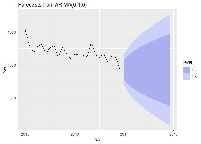
f_arima_multi <- m_arima %>%
  forecast(h = size)

f_arima_multi %>%
  autoplot()


# forecast ARIMA 2017 (Orininal Style)
f_arima<-forecast(m_arima,h=12)
f_arima %>%
  autoplot()


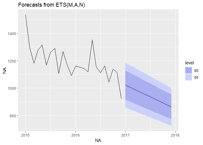
# forecast ETS 2017
f_ets = forecast(m_ets, h=12) 
f_ets %>%
  autoplot()


# check accuracy ETS
acc_ets <- accuracy(m_ets) 

#check accuracy ARIMA, between train and test sets
acc_arima_TrainVSTest <- accuracy(f_arima_multi, x = terror_byMonth_Test)

# check accuarcy ARIMA
acc_arima <- accuracy(f_arima)

# MAPE(ETS)= 20.03 < MAPE(ARIMA) = 22.05
# ETS model chosen 

# Compair to acctually 2017 data
accuracy(f_ets, terror_byMonth_Test)
#>                     ME      RMSE       MAE       MPE      MAPE      MASE
#> Training set -14.30982  90.08823  70.06438 -1.606862  5.900178 0.5790445
#> Test set     303.53575 316.03133 303.53575 23.986363 23.986363 2.5085599
#>                       ACF1 Theil's U
#> Training set  0.0008690031        NA
#> Test set     -0.2148651254  2.356116

Created on 2019-02-13 by the reprex package (v0.2.1)

This topic was automatically closed 21 days after the last reply. New replies are no longer allowed.

If you have a query related to it or one of the replies, start a new topic and refer back with a link.