Based on your dataset, I get the following:
library(package = "factoextra")
#> Loading required package: ggplot2
#> Welcome! Related Books: `Practical Guide To Cluster Analysis in R` at https://goo.gl/13EFCZ
dataset <- data.frame(Diversity = c(0.389838802, 1.459984531, 1.30710657, 0.695594724,
-1.138940812, -2.514842465, 0.695594724,
0.389838802, -0.374551005, 0.542716763, -0.374551005,
-0.068795083, -0.833184889, 0.848472686, -1.444696735,
0.848472686, 0.848472686, -0.068795083, -0.527428967,
-0.680306928),
AMBI = c(1.799252377, 0.777842731, 1.092122622, -0.793556725,
-0.872126698, 2.584952105, -1.029266644,
1.170692595, -0.164996943, -1.029266644, -0.243566916,
-0.714986753, -0.400706861, -0.243566916, -0.007856997,
-0.400706861, -0.243566916, 0.306422894, -0.714986753,
-0.872126698),
M_AMBI = c(-0.026636154, -0.026636154, 1.038809999, 1.038809999,
-1.624805383, -2.690251535, 0.506086922,
-0.55935923, -0.026636154, 0.506086922, 1.571533075, 0.506086922,
-0.55935923, 0.506086922, -1.092082306, 1.038809999,
0.506086922, -0.55935923, -0.026636154, -0.026636154),
TUBI = c(-0.46236525, -0.995863616, 0.426798692, 0.960297058,
-0.640198039, -1.529361981, 1.138129846,
0.604631481, 1.138129846, 1.315962635, 0.604631481, 0.782464269,
-0.284532462, -1.70719477, -1.70719477, 0.960297058,
0.071133115, -0.995863616, 0.604631481, -0.284532462),
BENTX = c(-1.658481729, -2.28432389, -1.479669682, -0.585609451,
1.023698965, 1.023698965, 1.023698965, 1.023698965,
0.219044757, 1.023698965, -0.675015474, -0.227985359,
1.023698965, 0.129638734, -0.138579336, 0.397856803,
-0.496203428, -0.406797405, 1.023698965, 0.04023271),
Temp = c(-3.601227684, 0.037718227, 0.037718227, 0.037718227,
0.037718227, -1.257107112, -1.257107112,
0.359072828, 0.359072828, 0.359072828, 0.359072828, 0.573067567,
0.573067567, 0.573067567, 0.573067567, 0.489348348,
0.489348348, 0.489348348, 0.489348348, 0.27861403),
DO = c(2.259516253, 2.259516253, 2.259516253, -0.311202851,
-0.311202851, 0.15011693, 0.15011693, -0.565351111,
-0.565351111, -0.565351111, -0.565351111,
-0.535109028, -0.535109028, -0.535109028, -0.535109028,
-0.504959428, -0.504959428, -0.504959428, -0.504959428,
-0.034698648),
TOC = c(1.075677765, 0.13235778, 1.583710696, -0.530378823,
1.152747528, 2.1278838, -1.097452336, 0.943481828,
0.199056672, -0.781167058, 0.360638279, -0.958518701,
-0.612067376, -0.004827845, -0.612067376, -1.193115427,
-1.193115427, 0.605099292, -1.193115427,
-0.004827845),
Chl_a = c(-0.096498665, -0.096498665, -0.096498665, -0.502949312,
-0.502949312, -0.160138841, -0.160138841,
-0.258498143, -0.258498143, -0.258498143, -0.258498143,
-0.771710385, -0.771710385, -0.771710385, -0.771710385,
1.824941493, 1.824941493, 1.824941493, 1.824941493,
-1.563259561))
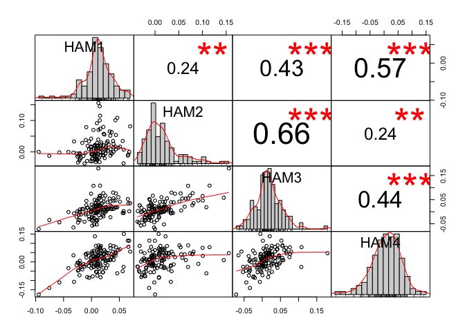
correlation_matrix_pearson <- cor(x = dataset,
method = "pearson")
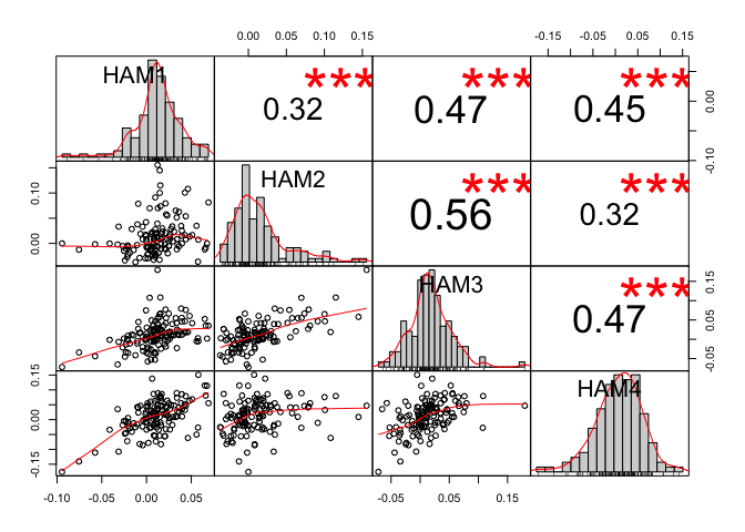
correlation_matrix_spearman <- cor(x = dataset,
method = "spearman")
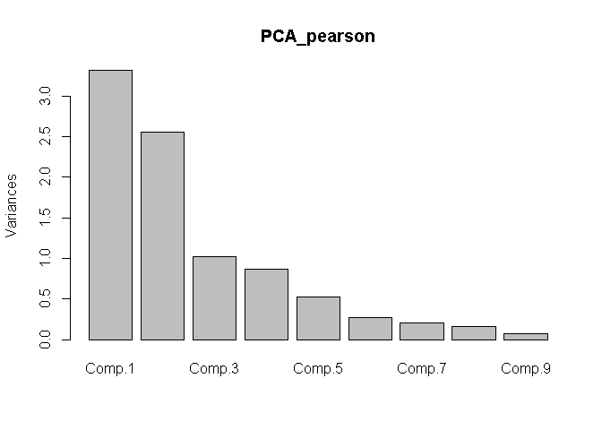
PCA_pearson <- princomp(covmat = correlation_matrix_pearson)
PCA_spearman <- princomp(covmat = correlation_matrix_spearman)
PCA_pearson
#> Call:
#> princomp(covmat = correlation_matrix_pearson)
#>
#> Standard deviations:
#> Comp.1 Comp.2 Comp.3 Comp.4 Comp.5 Comp.6 Comp.7
#> 1.8208966 1.5987484 1.0082677 0.9331524 0.7267676 0.5200717 0.4542649
#> Comp.8 Comp.9
#> 0.4032037 0.2708624
#>
#> 9 variables and NA observations.
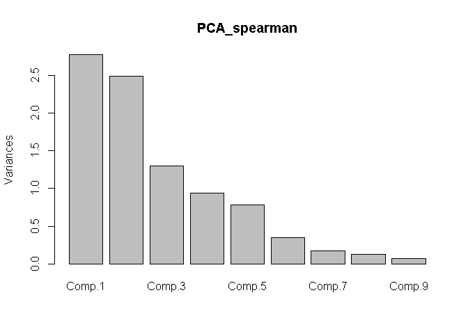
PCA_spearman
#> Call:
#> princomp(covmat = correlation_matrix_spearman)
#>
#> Standard deviations:
#> Comp.1 Comp.2 Comp.3 Comp.4 Comp.5 Comp.6 Comp.7
#> 1.6668773 1.5778042 1.1403007 0.9679142 0.8827371 0.5872683 0.4126256
#> Comp.8 Comp.9
#> 0.3576338 0.2695174
#>
#> 9 variables and NA observations.
plot(x = PCA_pearson)
plot(x = PCA_spearman)
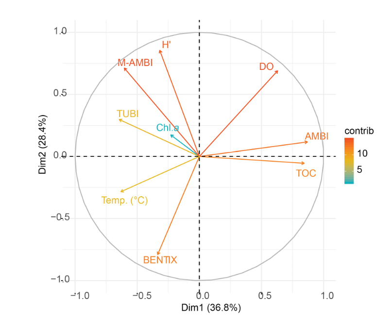
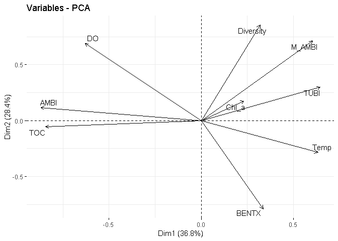
fviz_pca_var(X = PCA_pearson,
             repel = TRUE)
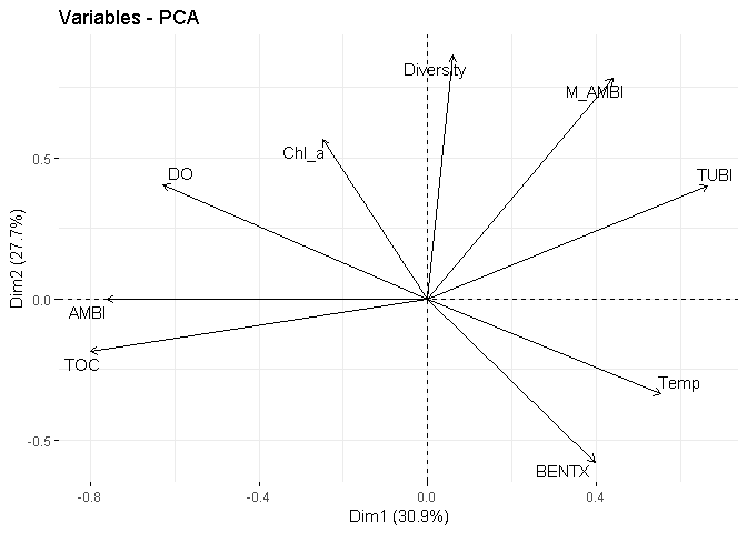
fviz_pca_var(X = PCA_spearman,
             repel = TRUE)
Created on 2019-03-15 by the reprex package (v0.2.1)