How to calculate the cumulative area of the overlapped normal distribution curve in R ?

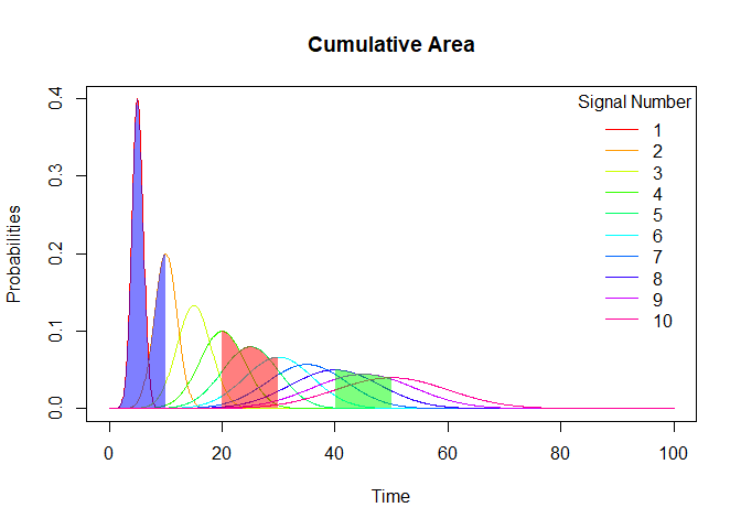
Please consider the below plot,
How can we calculate the area under each of the curves
under time = 1, 3, 5 and 7
Therefore, cumulative area at each interval

As it is not a standard plot, pnorm did not give this result for me

Basically, what % of the curve is covered at each interval
E.g,
Area of the 1st Signal at time = 5 is 50%
Area of Signal 2 at time = 10 is 50% but
What about at time = 1,3,5 and 7 for each of these signals ?

Does summation of y values until x interval is enough ?

mn <- 5
std <- 1.0
up_lmt <- max(1:10)*2*mn
st_ar = list()

for (i in 1:10) {
  st_ar[[i]] <- dnorm(x = seq(from = 0,to = up_lmt,length.out = 1e+3),
               mean = (i * mn),
               sd = i)
}

matplot(x = seq(from = 0,to = up_lmt,length.out = 1e+3),
        y = cbind(st_ar[[1]],st_ar[[2]],st_ar[[3]],
                  st_ar[[4]],st_ar[[5]],st_ar[[6]],
                  st_ar[[7]],st_ar[[8]],st_ar[[9]],
                  st_ar[[10]]),
        type = "l",
        lty = 1,
        col = c("violet","brown","pink","grey","blue","green","yellow","orange","red","black"),
        xlab = "Time",
        ylab = "Probabilities",
        main = "Cumulative area")
legend(x = "topright",
       title = "Signal number",
       legend = 1:10,
       col = c("violet","brown","pink","grey","blue","green","yellow","orange","red","black"),
       bty = "n",
       lty = 1)
Can you please elaborate? Which area do you want to find?

mn <- 5
std <- 1.0
up_lmt <- (max(1:10) * 2 * mn)

library(ggplot2)
library(purrr)

ggplot(data = data.frame(u = c(0, up_lmt)),
       mapping = aes(x = u)) +
  map(.x = 1:10,
      .f = ~ stat_function(mapping = aes(colour = paste("Distbn.", .x)),
                                     fun = dnorm,
                                     n = 1e+3,
                                     args = list(mean = (.x * mn),
                                                 sd = .x))) +
  scale_colour_manual(name = "Signal Number",
                      values = c("violet", "brown", "pink", "grey", "blue", "green", "yellow", "orange", "red", "black")) +
  labs(x = "Time",
       y = "Probabilities",
       title = "Cumulative Area")

Created on 2019-07-13 by the reprex package (v0.3.0)

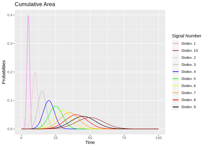
If I'm not too wrong, this is the same plot that your code produces. Can you please shade the portion area of which is your objective?

If you want to find the area under the \mathbb{N}(\mu, \sigma^2) density plot from -Inf to x, you use pnorm(x, \mu, \sigma). The area in between a and b, where a < b, is:

pnorm(b, \mu, \sigma) - pnorm(a, \mu, \sigma)

So, the area under the the curve of Signal i to the left of a point t and to the right of 0 will be pnorm(t, (i * mn), i) - pnorm(0, (i * mn), i). Does this help?

1 Like

Actually, trying to color all the area from all the curves to the left of
x = 10
polygon(c(x[x <= 10]), c(y[x <= 10]), col="red")

but it seems not functioning.

I had to retreat to familiar base graphics here, because my ggplot2 knowledge is exhausted. Maybe someone will show me a way to do these plots with ggplot. I guess I need to add a geom_area layer to my previous plot, but failed to do it properly.

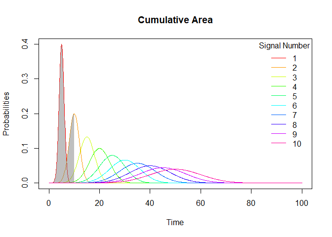
In the following reprex, I've showed how to plot the shaded region for the "maximum" curve (I don't know the proper terminology, but I hope the meaning is clear from the plot). What I understand from your description, this is your area of interest.

mean_sim <- 5
up_lmt <- (max(1:10) * 2 * mean_sim)

u <- seq(from = 0,
         to = up_lmt,
         length.out = 1e+3)
v <- sapply(X = 1:10,
            FUN = function(i) dnorm(x = u,
                                    mean = (i * mean_sim),
                                    sd = i))

matplot(x = u,
        y = v,
        type = "l",
        lty = 1,
        col = rainbow(n = 10),
        xlab = "Time",
        ylab = "Probabilities",
        main = "Cumulative Area")
legend(x = "topright",
       title = "Signal Number",
       legend = 1:10,
       col = rainbow(n = 10),
       bty = "n",
       lty = 1)

obj_pt <- 10
u_obj <- u[u <= obj_pt]
v_obj <- apply(X = v[(u <= obj_pt), ],
               MARGIN = 1,
               FUN = max)

polygon(x = c(0, u_obj, obj_pt),
        y = c(0, v_obj, 0),
        border = NA,
        col = rgb(red = 127.5,
                  green = 127.5,
                  blue = 127.5,
                  alpha = 127.5,
                  maxColorValue = 255))

library(DescTools)


AUC(x = c(0, u_obj, obj_pt),
    y = c(0, v_obj, 0))
#> [1] 1.401842

Created on 2019-07-13 by the reprex package (v0.3.0)

Hope this helps.

1 Like

Excellent solution @Yarnabrina

Final clarification on the topic:
How can we measure the area between time or x axis = 8 and 9 (basically not from origin)

Thanks for sharing the way to measure area from x axis = 0 to 10 below

But how about measuring intermediate values ?
i.e. Measuring area between x-axis: 8 and x-axis: 9
or between x-axis: 10 and x-axis: 19
which includes overlap of many curves

obj_pt <- 10
u_obj <- u[u <= obj_pt]
v_obj <- apply(X = v[(u <= obj_pt), ],
              MARGIN = 1,
              FUN = max)
AUC(x = c(0, u_obj, obj_pt),
   y = c(0, v_obj, 0))
mean_sim <- 5
up_lmt <- (max(1:10) * 2 * mean_sim)

u <- seq(from = 0,
         to = up_lmt,
         length.out = 1e+3)
v <- sapply(X = 1:10,
            FUN = function(i) dnorm(x = u,
                                    mean = (i * mean_sim),
                                    sd = i))

matplot(x = u,
        y = v,
        type = "l",
        lty = 1,
        col = rainbow(n = 10),
        xlab = "Time",
        ylab = "Probabilities",
        main = "Cumulative Area")
legend(x = "topright",
       title = "Signal Number",
       legend = 1:10,
       col = rainbow(n = 10),
       bty = "n",
       lty = 1)

shade_and_find_area <- function(start_pt, end_pt, colour = "grey")
{
  idx <- ((u >= start_pt) & (u <= end_pt))
  u_obj <- u[idx]
  v_obj <- apply(X = v[idx, ],
                 MARGIN = 1,
                 FUN = max)
  
  polygon(x = c(start_pt, u_obj, end_pt),
          y = c(0, v_obj, 0),
          border = NA,
          col = adjustcolor(col = colour,
                            alpha.f = 0.5))
  
  DescTools::AUC(x = c(start_pt, u_obj, end_pt),
                 y = c(0, v_obj, 0))
}

shade_and_find_area(start_pt = 0,
                    end_pt = 10,
                    colour = "blue")
#> [1] 1.401842

shade_and_find_area(start_pt = 20,
                    end_pt = 30,
                    colour = "red")
#> [1] 0.7824488

shade_and_find_area(start_pt = 40,
                    end_pt = 50,
                    colour = "green")
 #> [1] 0.4452164

1 Like

Kudos Champ @Yarnabrina for helping booming R kids like me :slight_smile:

Perfect solution ...Hats off to u
Happy weekend

This topic was automatically closed 7 days after the last reply. New replies are no longer allowed.