| GT | Loss |
|---|---|
| Medium slender | 20.09236862 |
| Medium slender | 30.58071604 |
| Medium slender | 27.59242652 |
| Long slender | 30.15715463 |
| Long slender | 24.3670063 |
| Long slender | 25.17705553 |
| Long slender | 12.72271205 |
| Long slender | 22.77796233 |
| Long slender | 23.86436103 |
| Medium slender | 36.59312563 |
| Medium slender | 36.69062323 |
| Medium slender | 38.66469706 |
| Long slender | 26.55925794 |
| Long slender | 24.19161441 |
| Long slender | 29.29602277 |
| Medium bold | 36.7456361 |
| Medium bold | 42.77148693 |
| Medium bold | 33.98163526 |
| Medium bold | 26.91716105 |
| Medium bold | 33.48683195 |
| Medium bold | 24.81912791 |
| Long slender | 34.17761871 |
| Long slender | 24.9207415 |
| Long slender | 24.2537 |
| Long slender | 20.63239342 |
| Long slender | 16.2334569 |
| Long slender | 16.34207769 |
| Medium bold | 16.49523697 |
| Medium bold | 12.02333522 |
| Medium bold | 13.09286917 |
| Long bold | 27.15206913 |
| Long bold | 19.57430573 |
| Long bold | 25.9421092 |
| Medium slender | 26.78612859 |
| Medium slender | 35.23848425 |
| Medium slender | 31.32410893 |
| Long bold | 25.64685947 |
| Long bold | 28.98320755 |
| Long bold | 24.33324921 |
| Medium bold | 24.64919266 |
| Medium bold | 27.77870313 |
| Medium bold | 34.42350877 |
| Medium bold | 24.45873167 |
| Medium bold | 26.89426315 |
| Medium bold | 20.03641169 |
| Long slender | 26.8545126 |
| Long slender | 25.83729063 |
| Long slender | 24.49976519 |
| Long bold | 21.41046872 |
| Long bold | 23.92436139 |
| Long bold | 23.38619827 |
| Long bold | 15.14173697 |
| Long bold | 14.4683789 |
| Long bold | 14.01994278 |
| Short bold | 28.71111512 |
| Short bold | 26.35626341 |
| Short bold | 28.58266541 |
| Long slender | 17.54578151 |
| Long slender | 14.75023306 |
| Long slender | 18.76527064 |
| Medium bold | 20.32031186 |
| Medium bold | 25.70571108 |
| Medium bold | 28.92054676 |
| Long slender | 27.22203267 |
| Long slender | 29.44174984 |
| Long slender | 24.84816034 |
| Medium bold | 28.83734269 |
| Medium bold | 30.51775973 |
| Medium bold | 31.33924009 |
| Medium bold | 22.77310814 |
| Medium bold | 26.94960759 |
| Medium bold | 30.35638389 |
| Long slender | 35.34899162 |
| Long slender | 42.49641671 |
| Long slender | 39.33831049 |
| Medium slender | 20.35001925 |
| Medium slender | 27.35150243 |
| Medium slender | 27.68193808 |
| Medium bold | 25.61599487 |
| Medium bold | 26.30567008 |
| Medium bold | 19.2320047 |
| Medium bold | 16.30728097 |
| Medium bold | 21.85078762 |
| Medium bold | 20.40250072 |
| Medium bold | 25.49497794 |
| Medium bold | 23.35183006 |
| Medium bold | 33.58038823 |
| Medium slender | 27.0812478 |
| Medium slender | 26.97539195 |
| Medium slender | 23.88487049 |
| Long slender | 26.0060857 |
| Long slender | 24.59684541 |
| Long slender | 29.41198635 |
| Medium bold | 31.62727653 |
| Medium bold | 34.44118036 |
| Medium bold | 32.32758272 |
| Long slender | 33.55150247 |
| Long slender | 37.83831887 |
| Long slender | 33.24723841 |
| Short bold | 26.28748748 |
| Short bold | 23.68686632 |
| Short bold | 27.7284831 |
| Medium bold | 22.89794871 |
| Medium bold | 28.04506867 |
| Medium bold | 25.73401175 |
| Medium bold | 29.22088207 |
| Medium bold | 31.51963118 |
| Medium bold | 27.81072195 |
| Long slender | 24.68435924 |
| Long slender | 30.68108761 |
| Long slender | 23.94852527 |
| Medium bold | 29.00451736 |
| Medium bold | 29.77237174 |
| Medium bold | 30.8210907 |
| Medium bold | 25.86727638 |
| Medium bold | 28.93491185 |
| Medium bold | 30.45260299 |
| Medium bold | 36.76278541 |
| Medium bold | 38.18164724 |
| Medium bold | 33.8426985 |
| Medium slender | 36.91166578 |
| Medium slender | 40.44140903 |
| Medium slender | 40.37268439 |
| Medium bold | 22.3970719 |
| Medium bold | 39.50420376 |
| Medium bold | 28.722364 |
| Medium bold | 22.53440666 |
| Medium bold | 30.40673993 |
| Medium bold | 27.99414054 |
| Medium bold | 31.62854324 |
| Medium bold | 31.57498296 |
| Medium bold | 29.76340677 |
| Medium bold | 26.17834721 |
| Medium bold | 24.49437256 |
| Medium bold | 25.93455705 |
| Long slender | 25.38467058 |
| Long slender | 31.82556156 |
| Long slender | 31.50345785 |
I used the following codes to compute p values and generate the plot
library(readxl)
Data<-read_excel("Speciation_rrr.xlsx", sheet = "Sheet2")
Data
library(tidyverse)
library(rstatix)
library(ggpubr)
library(ggplot2)
library(scales)
library(RColorBrewer)
compare_means(Loss ~ GT,  data = Data, p.adjust.method = "bonferroni")
my_comparisons <- list(c("Long bold", "Long slender"),
                       c("Long slender", "Medium bold"),
                       c("Medium bold", "Medium slender"),
                       c("Medium slender", "Short bold"))
GT <- ggplot(Data, aes(x = GT,y = Loss, fill= GT))+
  geom_boxplot(outlier.size = 1.5, outlier.shape = 21, fatten=1.5) +
  stat_boxplot(geom = "errorbar", width = 0.2, color="black",
               position = position_dodge(0.75)) +
  scale_fill_brewer(palette = "Set2")+
  stat_summary(fun = mean,geom = "point", shape = 16, size = 2.0,
               position = position_dodge(0.75))+
  scale_y_continuous(limits=c(0,70), breaks = seq(0,70,10))+
  scale_x_discrete(labels=c('Long bold\n(n=4)', 'Long slender\n(n=13)', 'Medium bold\n(n=21)',
                            'Medium slender\n(n=6)','Short bold\n(n=2)'))+
  labs(y=expression("%loss of total As"),
       x= Grain~size~and ~shape~classification)+
  theme_classic()+
  theme(legend.position = "none")+
  theme(panel.border = element_rect(color = "black", fill = NA,
                                    linewidth = 0.5))+
  theme(axis.title.x = element_text(face = "bold", color = "black",size = 8))+
  theme(axis.title.y = element_text(face = "bold", color = "black",size = 8))+
  theme(axis.text.x = element_text(color = "black",size = 8, angle =45, hjust=1))+
  theme(axis.text.y = element_text(color = "black",size = 8))+
  theme(axis.ticks.length = unit(-0.8, "mm"))+
  stat_compare_means(label.x = c(1.2))+
  stat_compare_means(comparisons = my_comparisons)


GT
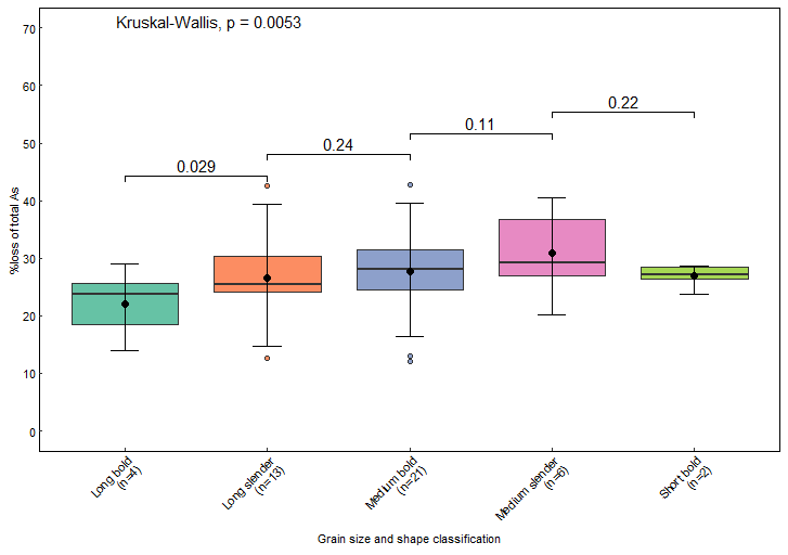
But I want the adjusted p values. Please help.