How do you draw such a diagram in code with the following data?

yuyu1 · December 4, 2024, 8:17am

dput(EC_2021_ASPR)
structure(list(year = 1990:2021, val = c(22.7, 22.7, 22.7, 22.5, 
22.2, 21.9, 21.4, 20.9, 20.4, 19.9, 19.6, 19.2, 18.7, 18.2, 17.8, 
17.3, 16.9, 16.4, 15.9, 15.5, 15.2, 15, 14.8, 14.5, 14.3, 14.1, 
13.9, 13.6, 13.4, 13.2, 13.7, 13.7), upper = c(31.8, 31.7, 31.4, 
31.1, 30.7, 30.2, 29.7, 29, 28.2, 27.7, 27.3, 26.9, 26.3, 25.6, 
25, 24.4, 23.7, 23, 22.2, 21.6, 21.2, 20.9, 20.6, 20.3, 20, 19.7, 
19.4, 19, 18.7, 18.5, 19.1, 19.1), lower = c(15.9, 16, 16, 15.9, 
15.7, 15.5, 15.2, 14.9, 14.5, 14.2, 13.9, 13.7, 13.3, 12.9, 12.5, 
12.2, 11.8, 11.5, 11.1, 10.8, 10.6, 10.5, 10.3, 10.2, 10, 9.9, 
9.8, 9.6, 9.5, 9.4, 9.7, 9.7), lower_to_upper = c("(15.9 to 31.8)", 
"(16 to 31.7)", "(16 to 31.4)", "(15.9 to 31.1)", "(15.7 to 30.7)", 
"(15.5 to 30.2)", "(15.2 to 29.7)", "(14.9 to 29)", "(14.5 to 28.2)", 
"(14.2 to 27.7)", "(13.9 to 27.3)", "(13.7 to 26.9)", "(13.3 to 26.3)", 
"(12.9 to 25.6)", "(12.5 to 25)", "(12.2 to 24.4)", "(11.8 to 23.7)", 
"(11.5 to 23)", "(11.1 to 22.2)", "(10.8 to 21.6)", "(10.6 to 21.2)", 
"(10.5 to 20.9)", "(10.3 to 20.6)", "(10.2 to 20.3)", "(10 to 20)", 
"(9.9 to 19.7)", "(9.8 to 19.4)", "(9.6 to 19)", "(9.5 to 18.7)", 
"(9.4 to 18.5)", "(9.7 to 19.1)", "(9.7 to 19.1)"), ASPR = c("22.7 (15.9 to 31.8)", 
"22.7 (16 to 31.7)", "22.7 (16 to 31.4)", "22.5 (15.9 to 31.1)", 
"22.2 (15.7 to 30.7)", "21.9 (15.5 to 30.2)", "21.4 (15.2 to 29.7)", 
"20.9 (14.9 to 29)", "20.4 (14.5 to 28.2)", "19.9 (14.2 to 27.7)", 
"19.6 (13.9 to 27.3)", "19.2 (13.7 to 26.9)", "18.7 (13.3 to 26.3)", 
"18.2 (12.9 to 25.6)", "17.8 (12.5 to 25)", "17.3 (12.2 to 24.4)", 
"16.9 (11.8 to 23.7)", "16.4 (11.5 to 23)", "15.9 (11.1 to 22.2)", 
"15.5 (10.8 to 21.6)", "15.2 (10.6 to 21.2)", "15 (10.5 to 20.9)", 
"14.8 (10.3 to 20.6)", "14.5 (10.2 to 20.3)", "14.3 (10 to 20)", 
"14.1 (9.9 to 19.7)", "13.9 (9.8 to 19.4)", "13.6 (9.6 to 19)", 
"13.4 (9.5 to 18.7)", "13.2 (9.4 to 18.5)", "13.7 (9.7 to 19.1)", 
"13.7 (9.7 to 19.1)")), row.names = c(1730L, 1732L, 1734L, 1736L, 
1738L, 1740L, 1742L, 1744L, 1746L, 1748L, 1750L, 1752L, 1754L, 
1756L, 1758L, 1760L, 1762L, 1764L, 1766L, 1768L, 1770L, 1772L, 
1774L, 1776L, 1778L, 1780L, 1782L, 1784L, 1786L, 1788L, 1790L, 
1792L), class = "data.frame")

微信图片_20241204161703

craig.parylo · December 4, 2024, 8:55am

Hi @yuyu1 ,

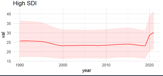
{ggplot2} is used here to plot the data in EC_2021_ASPR with year on the x-axis, val forming the main line plot. The using upper and lower bounds used for y_min and y_max in geom_ribbon to produce the shaded area.

library(ggplot2)
EC_2021_ASPR <-
  structure(list(year = 1990:2021, val = c(22.7, 22.7, 22.7, 22.5, 
                                           22.2, 21.9, 21.4, 20.9, 20.4, 19.9, 19.6, 19.2, 18.7, 18.2, 17.8, 
                                           17.3, 16.9, 16.4, 15.9, 15.5, 15.2, 15, 14.8, 14.5, 14.3, 14.1, 
                                           13.9, 13.6, 13.4, 13.2, 13.7, 13.7), upper = c(31.8, 31.7, 31.4, 
                                                                                          31.1, 30.7, 30.2, 29.7, 29, 28.2, 27.7, 27.3, 26.9, 26.3, 25.6, 
                                                                                          25, 24.4, 23.7, 23, 22.2, 21.6, 21.2, 20.9, 20.6, 20.3, 20, 19.7, 
                                                                                          19.4, 19, 18.7, 18.5, 19.1, 19.1), lower = c(15.9, 16, 16, 15.9, 
                                                                                                                                       15.7, 15.5, 15.2, 14.9, 14.5, 14.2, 13.9, 13.7, 13.3, 12.9, 12.5, 
                                                                                                                                       12.2, 11.8, 11.5, 11.1, 10.8, 10.6, 10.5, 10.3, 10.2, 10, 9.9, 
                                                                                                                                       9.8, 9.6, 9.5, 9.4, 9.7, 9.7), lower_to_upper = c("(15.9 to 31.8)", 
                                                                                                                                                                                         "(16 to 31.7)", "(16 to 31.4)", "(15.9 to 31.1)", "(15.7 to 30.7)", 
                                                                                                                                                                                         "(15.5 to 30.2)", "(15.2 to 29.7)", "(14.9 to 29)", "(14.5 to 28.2)", 
                                                                                                                                                                                         "(14.2 to 27.7)", "(13.9 to 27.3)", "(13.7 to 26.9)", "(13.3 to 26.3)", 
                                                                                                                                                                                         "(12.9 to 25.6)", "(12.5 to 25)", "(12.2 to 24.4)", "(11.8 to 23.7)", 
                                                                                                                                                                                         "(11.5 to 23)", "(11.1 to 22.2)", "(10.8 to 21.6)", "(10.6 to 21.2)", 
                                                                                                                                                                                         "(10.5 to 20.9)", "(10.3 to 20.6)", "(10.2 to 20.3)", "(10 to 20)", 
                                                                                                                                                                                         "(9.9 to 19.7)", "(9.8 to 19.4)", "(9.6 to 19)", "(9.5 to 18.7)", 
                                                                                                                                                                                         "(9.4 to 18.5)", "(9.7 to 19.1)", "(9.7 to 19.1)"), ASPR = c("22.7 (15.9 to 31.8)", 
                                                                                                                                                                                                                                                      "22.7 (16 to 31.7)", "22.7 (16 to 31.4)", "22.5 (15.9 to 31.1)", 
                                                                                                                                                                                                                                                      "22.2 (15.7 to 30.7)", "21.9 (15.5 to 30.2)", "21.4 (15.2 to 29.7)", 
                                                                                                                                                                                                                                                      "20.9 (14.9 to 29)", "20.4 (14.5 to 28.2)", "19.9 (14.2 to 27.7)", 
                                                                                                                                                                                                                                                      "19.6 (13.9 to 27.3)", "19.2 (13.7 to 26.9)", "18.7 (13.3 to 26.3)", 
                                                                                                                                                                                                                                                      "18.2 (12.9 to 25.6)", "17.8 (12.5 to 25)", "17.3 (12.2 to 24.4)", 
                                                                                                                                                                                                                                                      "16.9 (11.8 to 23.7)", "16.4 (11.5 to 23)", "15.9 (11.1 to 22.2)", 
                                                                                                                                                                                                                                                      "15.5 (10.8 to 21.6)", "15.2 (10.6 to 21.2)", "15 (10.5 to 20.9)", 
                                                                                                                                                                                                                                                      "14.8 (10.3 to 20.6)", "14.5 (10.2 to 20.3)", "14.3 (10 to 20)", 
                                                                                                                                                                                                                                                      "14.1 (9.9 to 19.7)", "13.9 (9.8 to 19.4)", "13.6 (9.6 to 19)", 
                                                                                                                                                                                                                                                      "13.4 (9.5 to 18.7)", "13.2 (9.4 to 18.5)", "13.7 (9.7 to 19.1)", 
                                                                                                                                                                                                                                                      "13.7 (9.7 to 19.1)")), row.names = c(1730L, 1732L, 1734L, 1736L, 
                                                                                                                                                                                                                                                                                            1738L, 1740L, 1742L, 1744L, 1746L, 1748L, 1750L, 1752L, 1754L, 
                                                                                                                                                                                                                                                                                            1756L, 1758L, 1760L, 1762L, 1764L, 1766L, 1768L, 1770L, 1772L, 
                                                                                                                                                                                                                                                                                            1774L, 1776L, 1778L, 1780L, 1782L, 1784L, 1786L, 1788L, 1790L, 
                                                                                                                                                                                                                                                                                            1792L), class = "data.frame")
EC_2021_ASPR |> 
  ggplot(aes(x = year, y = val)) +
  geom_line(colour = 'red') + 
  geom_ribbon(aes(ymin = lower, ymax = upper), alpha = 0.1, fill = 'red') +
  theme_minimal()

^{Created on 2024-12-04 with reprex v2.1.1}

yuyu1 · December 4, 2024, 2:49pm

thank you.thank you.Have a good day!

yuyu1 · December 11, 2024, 6:57am

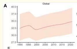
excuese me,could i have an additional question?I want to have a title such as"global" like my screen capture,how should I do?

craig.parylo · December 11, 2024, 8:18am

Hi @yuyu1 ,

Use can use the labs() function to add things like titles

yuyu1 · December 11, 2024, 3:32pm

thanks.I successfully made this graph using the code you told me but when I tried it just now it showed an error in the select function. I don't know why. Additionally, I added the title, is it correct to use the labs function this way?

library(ggplot2)
setwd('D:/Users/GBD数据')
EC <- read.csv('GBD_2021_DATAPI.csv',header = T)

EC_2021_ASPR <- subset(EC, 
                       EC$location=="High SDI"&
                         EC$age_name=='Age-standardized' & 
                         EC$sex_name=="Both"&
                         EC$metric_name== 'Rate' &
                         EC$measure_name=='Incidence')
#EC_2021_ASPR <- EC_2021_ASPR[,13:16]
val <- select(EC_2021_ASPR,val)
upper <- select(EC_2021_ASPR,upper)
lower <- select(EC_2021_ASPR,lower)
EC_2021_ASPR |> 
  ggplot(aes(x = year, y = val)) +
  geom_line(colour = 'red') + 
  geom_ribbon(aes(ymin = lower, ymax = upper), alpha = 0.1, fill = 'red') +
  theme_minimal()
labs(,title="High SDI")

val <- select(EC_2021_ASPR,val)
错误于select(EC_2021_ASPR, val): 没有"select"这个函数

craig.parylo · December 11, 2024, 3:50pm

You're nearly there. You can add labs() to the plot using the plus + sign after theme_minimal():

EC_2021_ASPR |> 
  ggplot(aes(x = year, y = val)) +
  geom_line(colour = 'red') + 
  geom_ribbon(aes(ymin = lower, ymax = upper), alpha = 0.1, fill = 'red') +
  theme_minimal() + 
  labs(title = 'High SDI')

PS, you don't need to extract columns for val, upper and lower to their own variables for the plot. If you're using these for something else, then thats fine.

yuyu1 · December 11, 2024, 4:09pm

It worked, and the title appeared. Many, very much thank you for that. I would like to put this title in the middle above it. What should I do?

craig.parylo · December 11, 2024, 4:24pm

In {ggplot2} title and subtitle are left justified by default. To change this you can adjust the theme:

EC_2021_ASPR |> 
  ggplot(aes(x = year, y = val)) +
  geom_line(colour = 'red') + 
  geom_ribbon(aes(ymin = lower, ymax = upper), alpha = 0.1, fill = 'red') +
  theme_minimal() + 
  labs(title = 'High SDI') +
  theme(plot.title = element_text(hjust = 0.5))

where hjust = 0.5 indicates to centre the title halfway across the plot area.