How do I highlight one bar in a bar graph using ggplot2

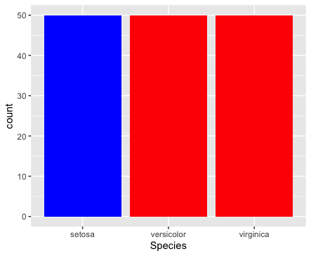
I'm trying to figure out how to highlight the "blue chips" bar in a bar chart. Please explain in the simplest way you can I am new to r. I am trying to make blue chips blue and everything else red.

library(readr)
library(dplyr)
library(tidyr)
library(stringr)
library(lubridate)
library(reprex)
library(tidyverse)
library(quantreg)
library(ggplot2)

sports_top25000 <- read.csv('index_sales_export_categories.csv') %>%
  select(graded_title, vcp_card_grade_id, category, year, date, price) %>%
  group_by(graded_title,vcp_card_grade_id,year) %>%
  summarise(Market_Cap = sum(price),Average_Price = mean(price),count=n(),
            Standard_Deviation = sd(price),SD_over_Price = (Standard_Deviation/Average_Price))
sports_top25000


sports_SD_over_Price <- sports_top25000$SD_over_Price
mean_sports_SD_over_Price <- mean(sports_SD_over_Price)


SD_over_Price_df <- data.frame("Card Type" = c("Blue Chips", 
                                              "All Sports", 
                                              "Baseball", 
                                              "Basketball", 
                                              "Football", 
                                              "Hockey",
                                              "Michael Jordan",
                                              "Mickey Mantle", 
                                              "Modern Baseball", 
                                              "Modern Basketball", 
                                              "Modern Football",
                                              "Postwar Baseball",
                                              "Postwar Hockey",
                                              "Prewar Baseball", 
                                              "Prewar Hockey", 
                                              "Vintage Basketball", 
                                              "Vintage Football"),
                               "Variability" = c(mean_blue_chips_sd_over_avg, 
                                              mean_sports_SD_over_Price,
                                              mean_baseball_SD_over_Price,
                                              mean_basketball_SD_over_Price, 
                                              mean_football_SD_over_Price,
                                              mean_hockey_SD_over_Price,
                                              mean_michael_jordan_basketball_SD_over_Price,
                                              mean_mickey_mantle_baseball_SD_over_Price,
                                              mean_modern_baseball_SD_over_Price,
                                              mean_modern_basketball_SD_over_Price,
                                              mean_modern_football_SD_over_Price,
                                              mean_postwar_baseball_SD_over_Price,
                                              mean_postwar_hockey_SD_over_Price,
                                              mean_prewar_baseball_SD_over_Price,
                                              mean_prewar_hockey_SD_over_Price,
                                              mean_vintage_basketball_SD_over_Price,
                                              mean_vintage_football_SD_over_Price),
                              stringsAsFactors = FALSE)
SD_over_Price_df <- SD_over_Price_df[order(SD_over_Price_df$Variability),]
SD_over_Price_df$Card.Type <- factor(SD_over_Price_df$Card.Type, levels = SD_over_Price_df$Card.Type)
head(SD_over_Price_df)

variability_of_sales_bar_chart <- ggplot(SD_over_Price_df, aes(x = Card.Type, y=Variability, fill=area)) + 
  geom_bar(stat = "identity", width=.5) +
  scale_fill_manual(values=c("blue","red","red","red","red","red","red","red","red","red","red","red","red","red""red","red")) +
  labs(title = "Variability of Different Card Types") + 
  theme(axis.text.x = element_text(angle = 65, vjust = 0.6))
plot(variability_of_sales_bar_chart)

I don't have the data in your example, so here's an example with a built-in data frame. The basic idea is that you create a new grouping variable that has one value for the category you want to highlight, and a different value for all of the other categories. In the first example below, we create the new grouping variable within the aes function in ggplot. In the second example, we add the new grouping variable to the data frame before piping it into ggplot. The result is the same either way.

library(tidyverse)

iris %>% 
  ggplot(aes(Species, fill=ifelse(Species=="setosa", "A","B"))) + 
    geom_bar(show.legend=FALSE) +
    scale_fill_manual(values=c(A="blue", B="red"))

iris %>% 
  mutate(fill.var = ifelse(Species=="setosa", "A","B")) %>% 
  ggplot(aes(Species, fill=fill.var)) + 
    geom_bar(show.legend=FALSE) +
    scale_fill_manual(values=c(A="blue", B="red"))

Rplot

1 Like

The data is in the data frame that I created in the code. And the means are all just integers.

But we don't have access to index_sales_export_categories.csv.

OK thanks I'll figure it out.

Your code can also be shortened quite a bit. We can provide details once we have a data sample.

I'm not allowed to post the data.

All we need is a small sample of fake data with a structure similar to your real data and that will run with your code and illustrate your problem.

3 Likes

This topic was automatically closed 21 days after the last reply. New replies are no longer allowed.