How do I add other data (sets) to calibration curve??

[ellen552]

I'm very new to rstudio and need help adding data to a calibration curve. I'll attach my whole code and what the graph looks like so far.

data2 <- read.csv(choose.files())
data2
data3 <- read.csv(choose.files())
data3

library(ggplot2)
library(scales)

data2 <- data.frame(stringsAsFactors = FALSE, Concentration = c("0.1", "0.3", "0.6", "0.9", "1.0"), Absorbance = c(0.767, 0.805, 0.879, 0.925, 0.974))

ggplot(data = data2, aes(x = Concentration, y = Absorbance, group=1)) +
geom_point() + geom_smooth(method=lm, se = FALSE, colour = "black") +
ylim(0.7, 1.4)

(I had to make data frames for the axis values as X was categorical and specific values were needed)

data3 is 3 individual values:
Control - 0.857
Pre-treatment - 1.379
Post-treatment - 1.075

The values above are the absorbance of different samples (so can be placed on the y axis), but I can't figure out how to put them as points on the graph. They need to correlate with the x axis as this is the unknown value needed to be calculated from the calibration curve. Hopefully that makes sense???
I'd also like to add a main title to the graph and data labels for the 3 points I'm trying to add, but can't seem to do that either!

Any help would be really appreciated because I'm losing my mind trying to figure this out!!
Thanks in advance

[Matthias]

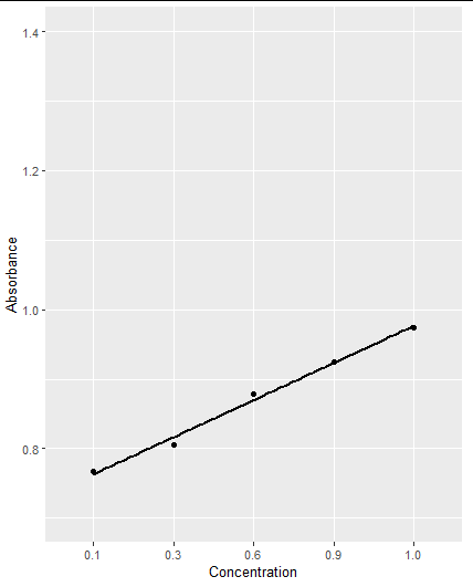
First of all, your data fr the x-axis need to be numeric!

data2 = data.frame(Concentration = c(0.1, 0.3, 0.6, 0.9, 1.0), 
                    Absorbance = c(0.767, 0.805, 0.879, 0.925, 0.974))

data3 = data.frame(Sample = c("Control", "Pre-treatment", "Post-treatment"),
                   Absorbance = c(0.857, 1.379, 1.075))

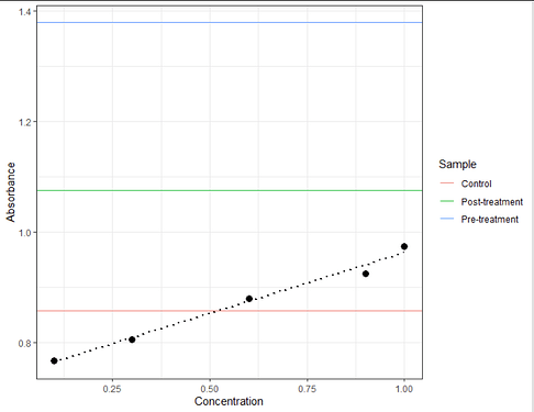
Then for the start you can just show the measured absorbances for the 3 samples as lines.
You see only control is within your calibration curve, post-treatment is a bit, pre-treatment massively outside.
This isn't good, as you don't know whether the trend remains linear or goes into a saturation.

#show the plot with readouts as line
ggplot(data = data2, 
       aes(x = Concentration, y = Absorbance)) +
  geom_point(size = 3) + 
  stat_smooth(method=lm, se = FALSE, 
              colour = "black", linetype = "dotted") + 
  theme_bw() + 
  geom_hline(data = data3, 
             aes(yintercept = Absorbance,
                 colour = Sample))

Then you can calculate a fit trough your values:

#calculate the linear fit
linear_fit=lm(Absorbance ~ Concentration, data = data2)
summary(linear_fit)
#
#Call:
#  lm(formula = Absorbance ~ Concentration, data = data2)
#
#Residuals:
#  1         2         3         4         5 
#0.002388 -0.003524  0.004609 -0.015259  0.011786 
#
#Coefficients:
#  Estimate Std. Error t value Pr(>|t|)    
#(Intercept)    0.74266    0.01029   72.20 5.86e-06 ***
#  Concentration  0.21956    0.01527   14.38 0.000729 ***
#  ---
#  Signif. codes:  0 ‘***’ 0.001 ‘**’ 0.01 ‘*’ 0.05 ‘.’ 0.1 ‘ ’ 1
#
#Residual standard error: 0.01171 on 3 degrees of freedom
#Multiple R-squared:  0.9857,	Adjusted R-squared:  0.9809 
#F-statistic: 206.9 on 1 and 3 DF,  p-value: 0.0007286

# good fit! 

# extract fitted (= expected) y values
linear_fit$fitted.values
#         1         2         3         4         5 
# 0.7646122 0.8085238 0.8743912 0.9402585 0.9622143
# this is quite close to what we put in

# extract the coeficicents
linear_fit$coefficients
#  (Intercept) Concentration 
# 0.7426565     0.2195578 

I am sure there must be a function to calculate x from y, for now I just found the opposite, predict calculates y from x. But we can do the math on our own and write a function for this:

# write a function to define x from given y
find_x = function(model, y) {
   # y = slope*x + intercept
   # y - intercept = slope*x
   # (y-intercept) / slope = x
   # just extract both values and do the math:
  intercept =  model$coefficients[1]
  slope = model$coefficients[2]
  x = (y-intercept)/slope
  return(x)  
}

# check with inputs
find_x(linear_fit, linear_fit$fitted.values)
#   1   2   3   4   5 
# 0.1 0.3 0.6 0.9 1.0
# okay works fine! 

# calculate for data3
find_x(linear_fit, data3$Absorbance)
# [1] 0.5207901 2.8982959 1.5136948

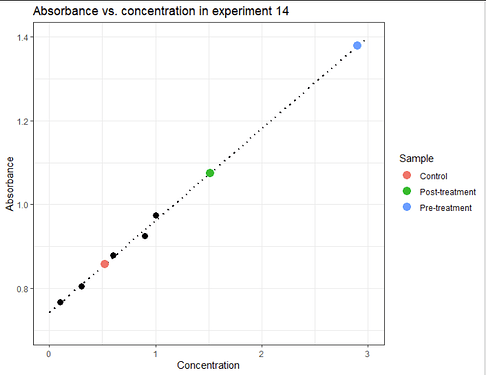
Ultimately we can add the results to data_3 and show the fitted results on the plot:

# add result to data3 
data3$Concentration = find_x(linear_fit, data3$Absorbance)

# plot again with points
ggplot(data = data2, 
       aes(x = Concentration, y = Absorbance)) +
  geom_smooth(method=lm, se = FALSE, 
              colour = "black", linetype = "dotted",
              fullrange = TRUE) + # to expnad it beyond the inputs
  geom_point(size = 3) +
  geom_point(data = data3,
             aes(colour = Sample),
             size = 4) + 
  ylim(0.7, 1.4) + xlim(0, 3) +
  theme_bw() + 
  labs(title = "Absorbance vs. concentration in experiment 14") # or whatever title you need