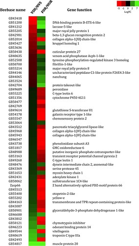
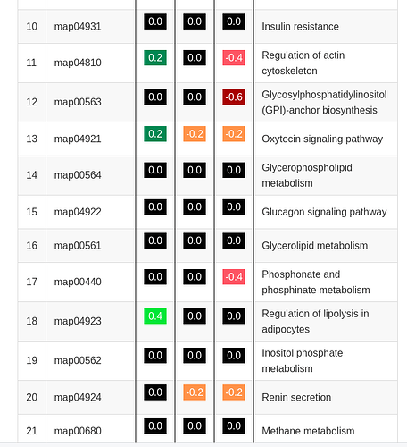
The reprex doesn't reproduce the colors, which are shown in the screenshot.
# libraries
library(classInt)
library(dplyr)
#>
#> Attaching package: 'dplyr'
#> The following objects are masked from 'package:stats':
#>
#>     filter, lag
#> The following objects are masked from 'package:base':
#>
#>     intersect, setdiff, setequal, union
library(ggplot2)
library(r2r)
library(htmlTable)
library(magrittr)
library(patchwork)
library(stringr)

# functions

# bin vector of numbers, x, into bins by y
bindh <- function (x, y) trunc(x/y) * y

# constants

# selected after selecting bins
bin_vector = c(0, 0.2, 0.4, -0.2, -0.4, -0.6)
# equal length to bin_vector
cols       = c("#000000", "#008751", "#00e636",
               "#ff9248", "#fd5463", "#a80000")
# used in constructing inline markup
forepart <- "<div style='background-color:"
midpart  <- "; color: white;'>"
aftpart  <- "</div>"

# data
Data <- data.frame(tibble::tribble(
  ~Beebase_name, ~Description, ~logFCJULVSAUG, ~logFCJULVSSEPT, ~logFCAUGVSSEPT,
  "map04932", "Non-alcoholic fatty liver disease", 0.075670032, 0.003935337, 0.01408051,
  "map00332", "Carbapenem biosynthesis", -0.014031521, 4.9e-05, -0.071734739,
  "map00333", "Prodigiosin biosynthesis", 0.007131704, 0.020343039, 0.013211291,
  "map04933", "AGE-RAGE signaling pathway in diabetic complications", 0.004932971, -0.051448915, -0.05638193,
  "map00330", "Arginine and proline metabolism", 0.010045605, -0.003979007, -0.014024656,
  "map04934", "Cushing syndrome", 0.010501308, -0.006209653, -0.016711005,
  "map00331", "Clavulanic acid biosynthesis", -0.066802306, -0.079918417, -0.013116154,
  "map00450", "Selenocompound metabolism", -0.002724964, -0.00292324, -0.000198,
  "map04930", "Type II diabetes mellitus", 0.004425738, -0.001000992, -0.005426774,
  "map04931", "Insulin resistance", -0.003641615, -0.000937, 0.002704848,
  "map04810", "Regulation of actin cytoskeleton", 0.316469292, -0.126381822, -0.442851157,
  "map00563", "Glycosylphosphatidylinositol (GPI)-anchor biosynthesis", 0.172221706, -0.074206148, -0.615193702,
  "map04921", "Oxytocin signaling pathway", 0.356132843, -0.259060815, -0.246427898,
  "map00564", "Glycerophospholipid metabolism", -0.012186907, -0.008827405, 0.003359457,
  "map04922", "Glucagon signaling pathway", 0.000999, -0.005950848, -0.006949856,
  "map00561", "Glycerolipid metabolism", 0.002776084, 0.005820994, 0.003044867,
  "map00440", "Phosphonate and phosphinate metabolism", 0.103317267, 0.05697387, -0.526828638,
  "map04923", "Regulation of lipolysis in adipocytes", 0.40709608, -0.119732514, -0.046343441,
  "map00562", "Inositol phosphate metabolism", 0.00227146, -0.006225672, -0.008497176,
  "map04924", "Renin secretion", 0.005229426, -0.313909259, -0.319138729,
  "map00680", "Methane metabolism", -0.002860128, 0.017217665, 0.020077748,
  "map04925", "Aldosterone synthesis and secretion", 0.113626918, -0.327363593, -0.440990554,
  "map04926", "Relaxin signaling pathway", 0.003958041, -0.095366001, -0.099324086,
  "map04927", "Cortisol synthesis and secretion", 0.125877766, -0.475589127, -0.601466936
))

# determine intervals to bin ratios of three variables
# this long section can be skipped if bins are known
# in advance

# one covers a mostly positive range and two cover mostly negative ranges
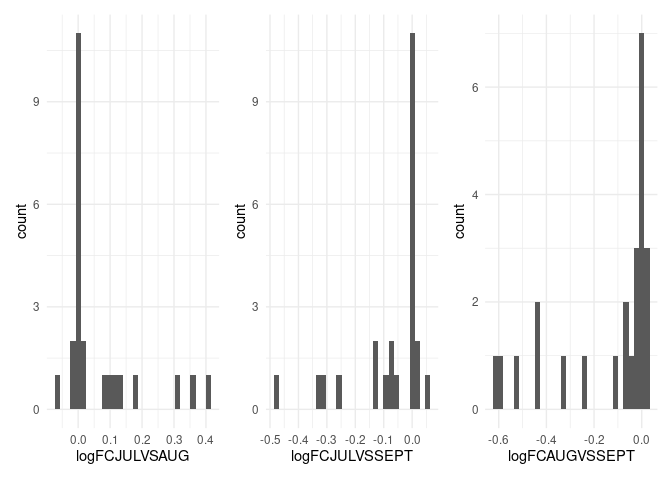
p1 <- ggplot(Data, aes(logFCJULVSAUG)) +
  geom_histogram() +
  theme_minimal()
p2 <- ggplot(Data, aes(logFCJULVSSEPT)) +
  geom_histogram() +
  theme_minimal()
p3 <- ggplot(Data, aes(logFCAUGVSSEPT)) +
  geom_histogram() +
  theme_minimal()

p1 + p2 + p3
#> `stat_bin()` using `bins = 30`. Pick better value with `binwidth`.
#> `stat_bin()` using `bins = 30`. Pick better value with `binwidth`.
#> `stat_bin()` using `bins = 30`. Pick better value with `binwidth`.

# find overall distribution

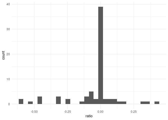
v <- data.frame(ratio = c(Data$logFCJULVSAUG, Data$logFCJULVSSEPT,
                          Data$logFCAUGVSSEPT))

p4 <- ggplot(v, aes(ratio)) +
  geom_histogram() +
  theme_minimal()

p4
#> `stat_bin()` using `bins = 30`. Pick better value with `binwidth`.

summary(v)
#>      ratio
#>  Min.   :-0.615194
#>  1st Qu.:-0.068035
#>  Median :-0.003282
#>  Mean   :-0.051519
#>  3rd Qu.: 0.005377
#>  Max.   : 0.407096

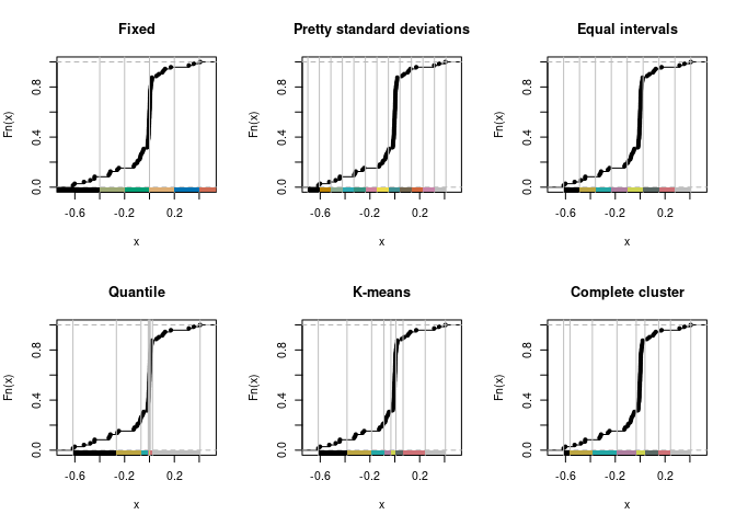
# adapted from classIntervals {classInt} example

pal1  <- c("#000000", "#E69F00", "#56B4E9", "#009E73", "#CC79A7",
           "#F0E442", "#0072B2", "#D55E00", "#CC79A7", "grey")
opar <- par(mfrow=c(2,3))
plot(classIntervals(v$ratio,
  style = "fixed",
  fixedBreaks = c(-0.8, -0.4, -0.2, 0, 0.2, 0.4, 0.6, 0.8)
), pal = pal1, main = "Fixed")
plot(classIntervals(v$ratio, style = "sd"), pal = pal1, main = "Pretty standard deviations")
plot(classIntervals(v$ratio, style = "equal"), pal = pal1, main = "Equal intervals")
set.seed(1)
plot(classIntervals(v$ratio, style = "quantile"), pal = pal1, main = "Quantile")

plot(classIntervals(v$ratio, style = "kmeans"), pal = pal1, main = "K-means")
plot(classIntervals(v$ratio, style = "hclust", method = "complete"),
  pal = pal1, main = "Complete cluster"
)

# unless there is a domain-specific reasons why breaks represent
# important state transitions, the fixed interval scale
# breaks appear best suited to bin the data

# end of determining bins

# preprocessing

# bin the data into increments of 0.2

# bin1 corresponds to logFCJULVSAUG, etc.
Data$bin1 <- bindh(Data$logFCJULVSAUG,0.2)
Data$bin2 <- bindh(Data$logFCJULVSSEPT,0.2)
Data$bin3 <- bindh(Data$logFCAUGVSSEPT,0.2)

# to keep Data intact, use subset for HTML required modifications
for_table <- Data[,c(1,2,6,7,8)]

# main

# create hash table (used in mutate())
ht <- hashmap()
# add colors
ht[bin_vector] <- cols

# add variables for color codes based on hash table
for_table <- for_table %>% mutate(color1 = ht[bin1],
                                  color2 = ht[bin2],
                                  color3 = ht[bin3])

# unknown cause: if bin3 is -0.6, color3 = ht[bin3] = NULL in
# mutate, but ht[-0.6] yields "#F0E442" correctly
# fix manually--an official kludge
for_table[12,8] <- "#a80000"
for_table[24,8] <- "#a80000"

# construct html markup variables and change 0 to display as 0.00

for_table %<>% mutate(cell1 = paste(forepart,color1,midpart,bin1,aftpart),
                     cell2 = paste(forepart,color2,midpart,bin2,aftpart),
                     cell3 = paste(forepart,color3,midpart,bin3,aftpart)) %>%
                     select(Beebase_name,cell1,cell2,cell3,Description) %>%
              mutate(cell1 = str_replace(cell1," 0 "," 0.0 "),
                     cell2 = str_replace(cell2," 0 "," 0.0 "),
                     cell3 = str_replace(cell3," 0 "," 0.0 "))


# render HTML table
# set column alignments
setHtmlTableTheme(align = "l|c|c|c|l")
htmlTable(for_table)
|
|
Beebase_name
|
cell1
|
cell2
|
cell3
|
Description
|
|
1
|
map04932
|
|
|
|
Non-alcoholic fatty liver disease
|
|
2
|
map00332
|
|
|
|
Carbapenem biosynthesis
|
|
3
|
map00333
|
|
|
|
Prodigiosin biosynthesis
|
|
4
|
map04933
|
|
|
|
AGE-RAGE signaling pathway in diabetic complications
|
|
5
|
map00330
|
|
|
|
Arginine and proline metabolism
|
|
6
|
map04934
|
|
|
|
Cushing syndrome
|
|
7
|
map00331
|
|
|
|
Clavulanic acid biosynthesis
|
|
8
|
map00450
|
|
|
|
Selenocompound metabolism
|
|
9
|
map04930
|
|
|
|
Type II diabetes mellitus
|
|
10
|
map04931
|
|
|
|
Insulin resistance
|
|
11
|
map04810
|
|
|
|
Regulation of actin cytoskeleton
|
|
12
|
map00563
|
|
|
|
Glycosylphosphatidylinositol (GPI)-anchor biosynthesis
|
|
13
|
map04921
|
|
|
|
Oxytocin signaling pathway
|
|
14
|
map00564
|
|
|
|
Glycerophospholipid metabolism
|
|
15
|
map04922
|
|
|
|
Glucagon signaling pathway
|
|
16
|
map00561
|
|
|
|
Glycerolipid metabolism
|
|
17
|
map00440
|
|
|
|
Phosphonate and phosphinate metabolism
|
|
18
|
map04923
|
|
|
|
Regulation of lipolysis in adipocytes
|
|
19
|
map00562
|
|
|
|
Inositol phosphate metabolism
|
|
20
|
map04924
|
|
|
|
Renin secretion
|
|
21
|
map00680
|
|
|
|
Methane metabolism
|
|
22
|
map04925
|
|
|
|
Aldosterone synthesis and secretion
|
|
23
|
map04926
|
|
|
|
Relaxin signaling pathway
|
|
24
|
map04927
|
|
|
|
Cortisol synthesis and secretion
|
